Lecture slides for GIS/MEA582

Spatial Interpolation: Splines

Helena Mitasova

GIS/MEA582 Geospatial Modeling and Analysis NCSU

Outline (learning objectives)

Spline interpolation
Spline parameters: tension and smoothing
Evaluating interpolation accuracy: deviations, crossvalidation
Special cases: contours, anisotropy
Processing large point data sets: segmentation, subsampling
Multivariate interpolation: volumes, topo-climatology, dynamic volumes

Interpolation with radial basis functions (RBF)

Variational approach is based on minimizing:
- deviations from the given points
- smoothness seminorm or roughness penalty
Radial basis functions: multiquadrics, splines
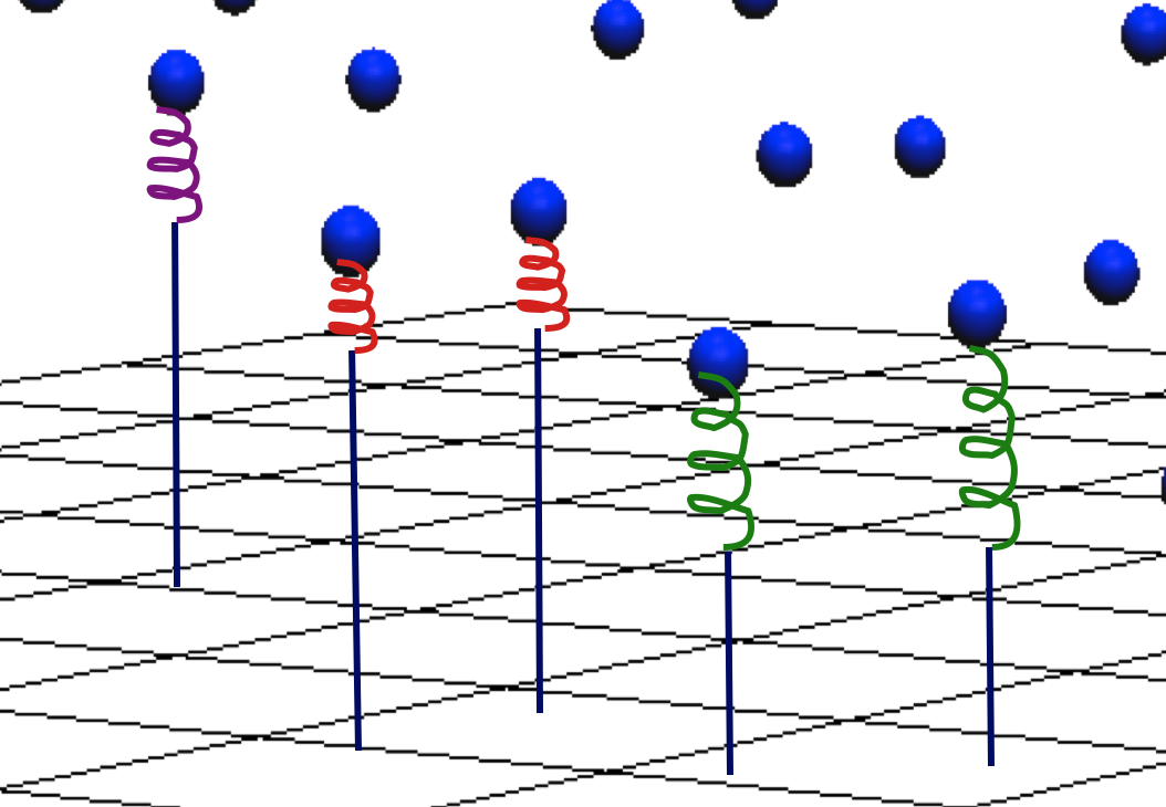
Physics-based interpretation: spline function is a thin flexible plate with tunable bending energy
Formally equivalent to universal kriging

Splines: general equation

$$ F(r) = T(r) + ∑ λ_j R(r,r_j) \; j=1,m $$

$r = (x,y)$ is location of a grid point,
$r_j=(x_j,y_j$) is location of a measured point
$λ_j$ are coefficients
$R(r,r_j)$ is a radial basis function
$T(r)$ is a trend:
low order polynomial: $a_0$, $a_0+a_1x+a_2y$, ...,

Splines with different properties

Spline properties depend on the formulation of smoothness seminorm or roughness penalty

thin plate spline ($2^{nd}$ order derivatives)
spline with tension ($1^{st}$ and $2^{nd}$ order derivatives)
regularized spline ($2^{nd}$ and higher order)
regularized spline with tension (derivatives of all orders with decreasing weight)
see the smoothness seminorms in Table 1
see example equations for $R(.)$ here

Note: Functions with $2^{nd}$ order derivatives minimize curvatures

Regularized spline with tension (RST)

$$ F(r) = T(r) + ∑ λ_j R(\varphi |r-r_j|) \; j=1,m $$

$\varphi$ is the tension parameter and
$|r-r_j|$ is the squared distance between the unsampled and measured points.
minimizes seminorm with all derivatives with decreasing weight

Spline tension rescales distances, it has similar effect to adjusting the range in kriging or the distance weight exponent in IDW

Spline: tension parameter

Tension controls the stiffness of the plate:

high tension: soft rubber sheet, short range
low tension: stiff steel plate, long range

Spline: tension parameter

High tension, short range of influence, soft rubber sheet, results in a rough surface with a peak or pit in each data point

Low tension, long range of influence, stiffer steel plate, results in a smoother surface with possible overshoots.

Note that tension is inverse of stiffness

Spline: smoothing parameter

Allows the surface to deviate from measured points

$$F(x_i,y_i) = z(x_i, y_i) + \varepsilon(x_i,y_i)$$

Reduces overshoots, smoothes out noise, improves numerical stability. It can be applied to individual points.

Spline: smoothing

Smoothing controls the deviation from the data points, large smoothing results in trend surface $T(x,y)$

Smoothing spline applied to concentrations of COVID-19 virus in wastewater

Spline: smoothing

Smoothing can be spatially variable

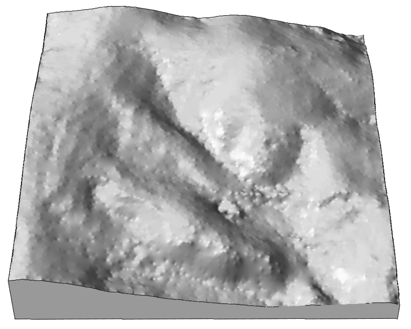
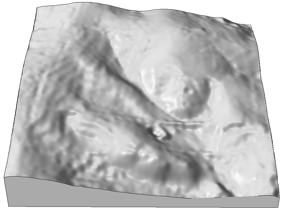
Spline implementations

Spline with tension: numerical solution supports carved streams, but here the tension is too high
Explicit RST method: lower tension combined with smoothing reduce bias towards given points

Figure from Mitas, L., Mitasova, H., 1999, Spatial Interpolation. In: P.Longley, M.F. Goodchild, D.J. Maguire, D.W.Rhind (Eds.), GIS: Principles, Techniques, Management and Applications, GeoInformation International, Wiley, 481-492.

Interpolation with anisotropy

Anisotropic tension: rescaling distances in a given direction changes the range of influence in this direction, leading to anisotropic pattern in the resulting surface

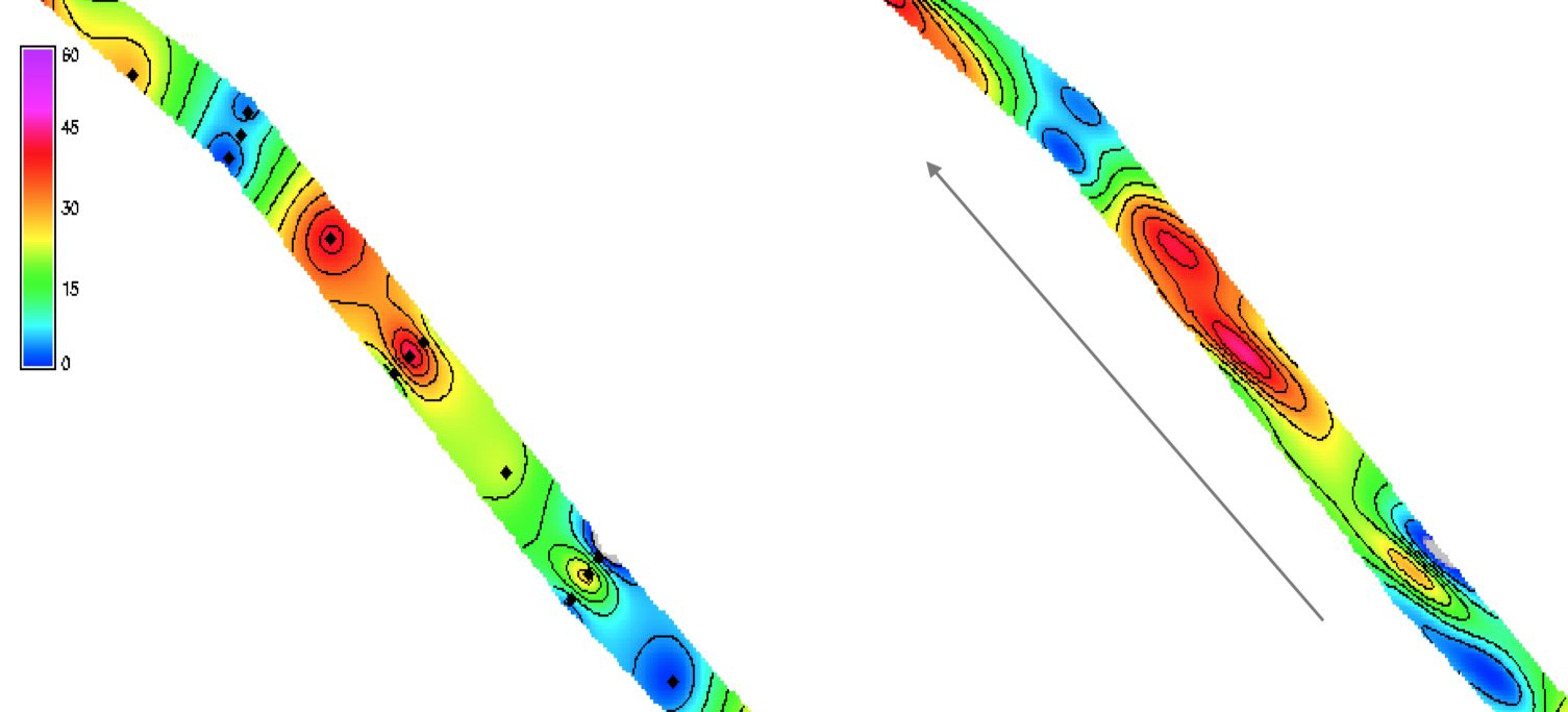
Data from Genereux, D.P., S. Leahy, H. Mitasova, C.D. Kennedy, and D.R. Corbett, 2008, Spatial and temporal variability of streambed hydraulic conductivity in West Bear Creek, NC, J. Hydrology, 358, p. 332-352

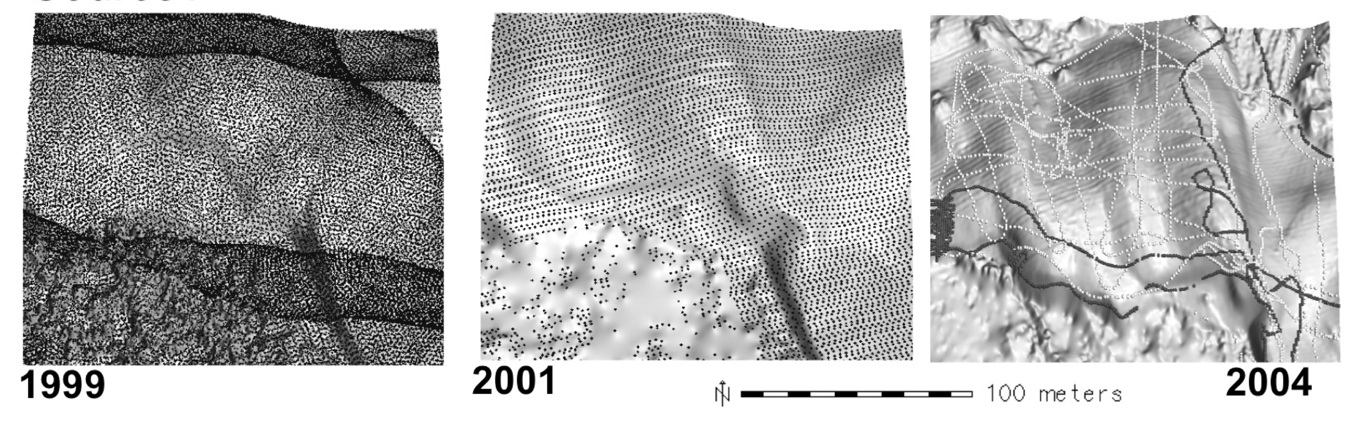
Interpolation from profiles

GPS-based sensors: dense sampling along a line
use anisotropy to rescale distances between profiles, minimize artifacts

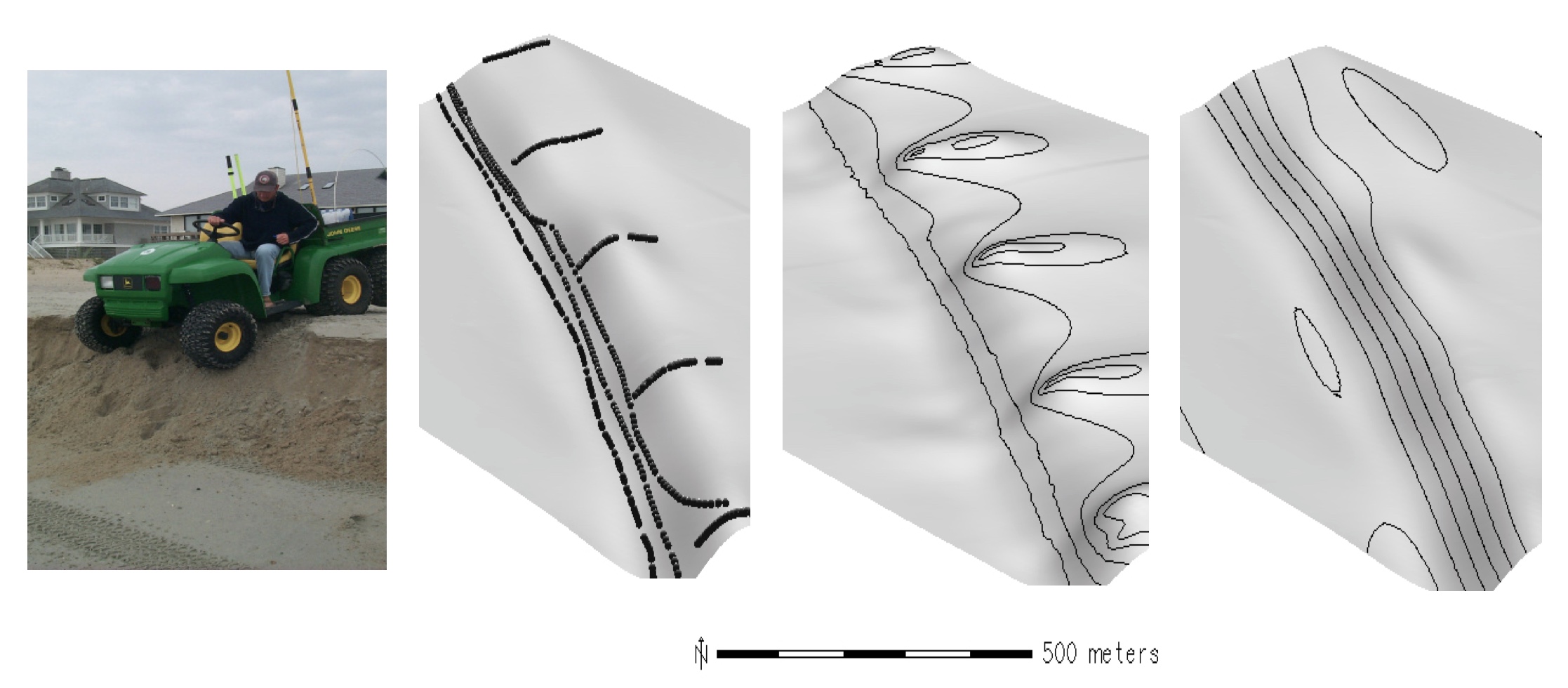
Better alternative is to map the beach with a drone using structure from motion

Interpolation accuracy

Effect of smoothing: deviations from given points $$ dz (x,y) = z' (x,y) – z (x,y) $$
where $z'$ is the interpolated value and $z$ is the given value
Predictive accuracy: crossvalidation error $$e_z (x,y) = z' (x,y) – z_o (x,y)$$
where $z'$ is the interpolated and $z_o$ is the given value in a point that was omitted from the set of points used for the interpolation. n-interpolations are performed, each time omitting one point in which $e_z$ is computed: also called leave-one-out cross-validation (LOOCV)
Artifacts, bias can be found using histograms, aspect maps, curvatures

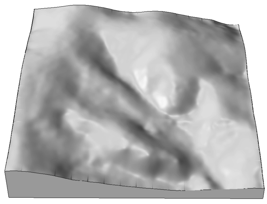
Interpolated surface deviations

Deviations map for smoothing 0.1 and 10

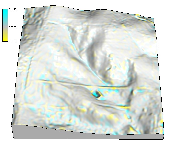
Color maps of differences between the given and interpolated values draped over the DEMs

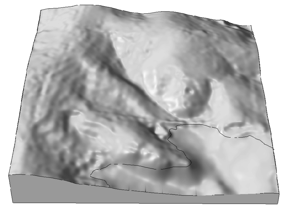
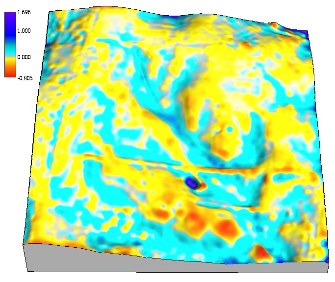
Interpolated surface predictive errors

Map showing spatial pattern of predictive errors

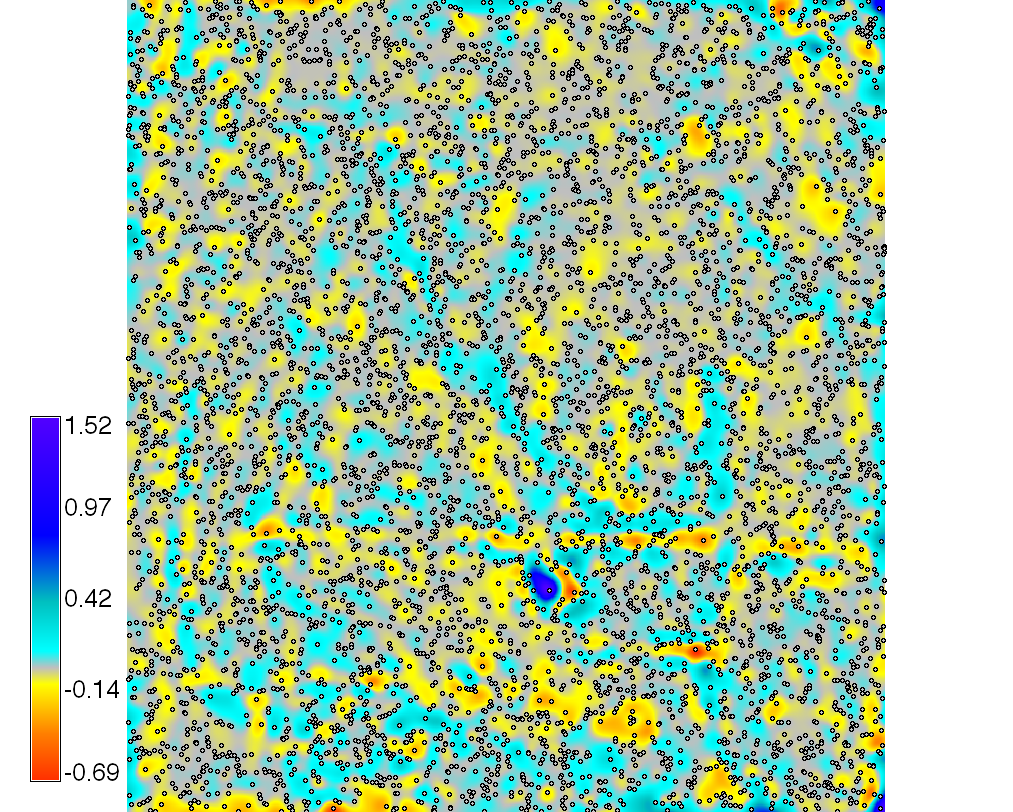
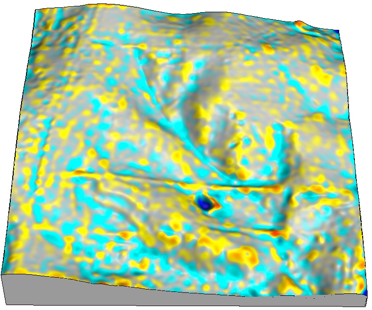
Map of differences between the interpolated and given values in a point that was omitted from the set of points used for the interpolation (leave one out cross-validation), shown with given set of points and draped over DEM.

Solutions for large data sets

Measured point data often include thousands to millions of points (point clouds)
To compute the coefficients of interpolation function we need to solve a system of $n$ linear equations, where $n$ is number of given points.
To keep $n$ small we compute interpolation locally with optimized search or apply segmented processing

Segmented processing

Segmented processing splits the region into rectagular segments
each rectangular segment has approximately same number of measured points
interpolation is performed for all grid points within the segment
interpolation function is computed using measured points within the segment and its neighborhood

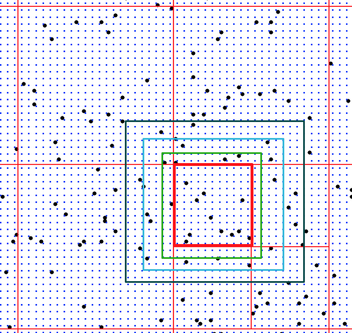
Quadtree segmentation

if the number of points within a rectangle is larger than given maximum, it is split into 4 smaller rectangles.
dynamic search window is used to find overlapping points to ensure smooth connection of segments

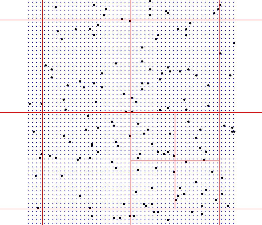
Quadtree segmentation

Interpolation of a river bathymetry using quadtree segmentation

Oversampling in point measurements

Automated point data acquisition often leads to large data sets with redundant points. Examples:

point clouds acquired by lidar
point data along profile collected automatically by GPS
scanned contours converted to points

Point density reduction

Can we interpolate a 2D grid if we have points with identical $x,y$ but different $z$?
How do we define identical?
minimum distance at which two points are considered two independent measurements (usually horizontal accuracy of the measured data)

We can eliminate points where $d_{i,j} > d_{min}$, usually $d_{min}$ is a function of data accuracy and grid resolution, often leading to much faster computation while preserving the level of detail.

Optimized subsampling

If the density of points along contours is high, spline with high tension leads to steps along contours. Solution:

Subsample points based on distance and shape.
Example: reduction from 40,000 to 3000 points - no visible change in isoline geometry

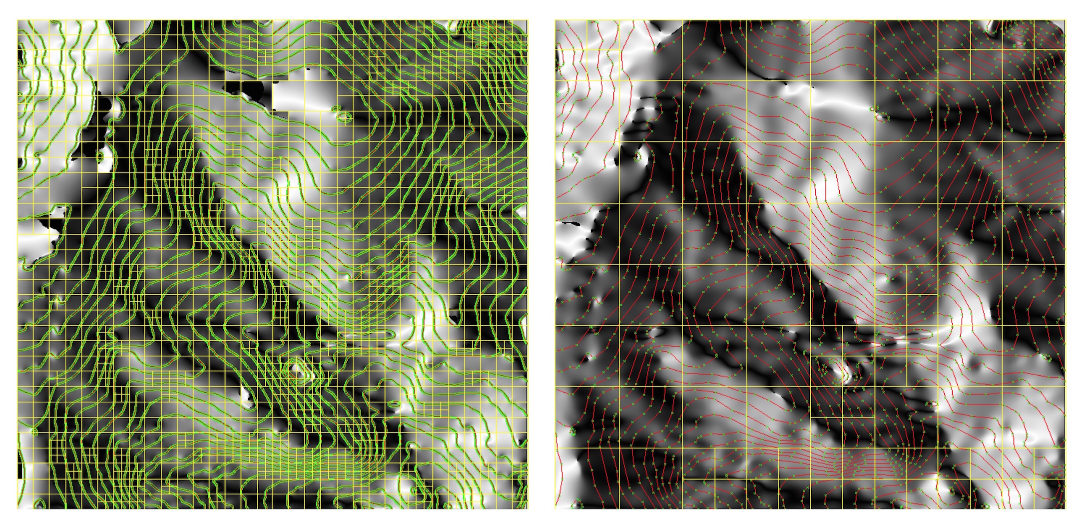
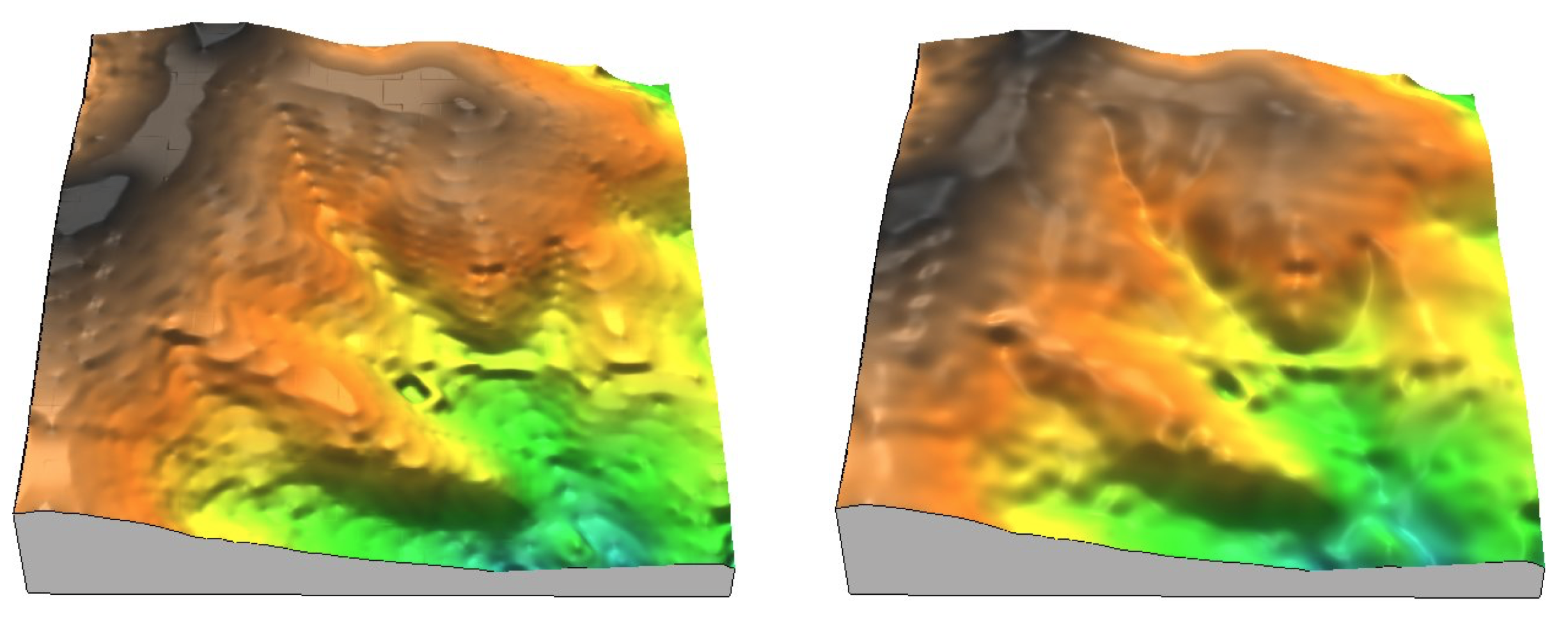
Interpolation with optimized subsampling

Point reduction and lower tension improves the result, while computation is 10-times faster with no artifacts

Subsampling lidar point clouds: 50-90% points can be often removed leading to much faster interpolation and fewer artifacts

Multivariate spline interpolation

Given $m$ points measured in 3D space, find such trivariate spline function $F(x,y,z$) that for each $i=1,m$ $$ w_i=F(x_i,y_i,z_i) $$
and compute $w_k=F(x_k,y_k,z_k)$ in 3D grid points
Similarly for points measured in 4D space (3D + time): $w_i=F(x_i,y_i,z_i,t_i)$
we use the quadvariate spline to compute a 4D grid (or a series of 3D grids)

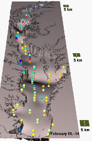
Trivariate Interpolation: volume

Nitrogen concentrations $w_i$ in the Chesapeake Bay sampled at points $(x_i,y_i,z_i)$ with different depths

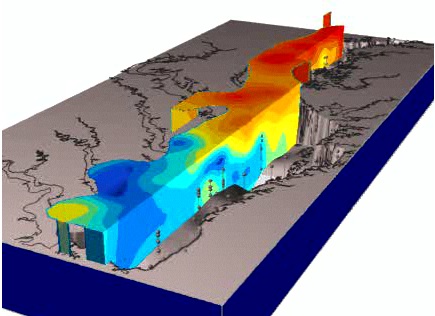
Trivariate Interpolation: tension

Impact of tension on the volume model: high to low

Mitas, L., Mitasova, H., 1999, Spatial Interpolation. GeoInformation International, Wiley, 481-492.

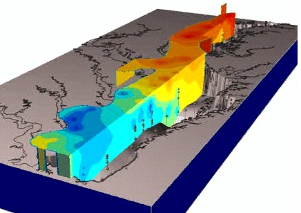
Trivariate Interpolation: tension

Impact of tension on the volume model

High tension: local maxima or minima at given points; low tension: smooth pattern with potential "overshoots"

Mitas, L., Mitasova, H., 1999, Spatial Interpolation. GeoInformation International, Wiley, 481-492.

Trivariate Interpolation to 2D grid

Interpolation of 2D grid with influence of third variable
Given $m$ points $(x_i,y_i,z_i,w_i)$ where $z_i = F_1 (x_i,y_i)$ find such $F_2(x,y,z)$ that for each $i=1,m$ $$ w_i=F_2(x_i,y_i,z_i) $$
then compute $w_k=F_3(x_k,y_k)$ at $F_1 \cap F_2$

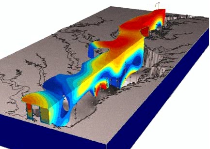
Example: $w_i$ is precipitation measured at locations $x_i,y_i$ at ground elevation $z_i$. $F_1$ is represented by a DEM, $F_2$ is an interpolated precipitation volume (voxel model) that passes through the points $(x_i,y_i,z_i,w_i)$. $F_3$ is a bivariate function represented as a 2D precipitation grid which is an intersection of a DEM and the interpolated precipitation volume $F_2$
Statistical approach of the method is described in Hutchinson, MF, 1995, Interpolating mean rainfall using thin plate smoothing splines, Int. Journal of Geographical Information Systems 9(4), 385-403. and has been used to interpolate global climate maps
See also Hofierka J., et al. 2002, Multivariate Interpolation of Precipitation Using Regularized Spline with Tension. TGIS 6(2), 135-150.

Trivariate Interpolation: precipitation

NC mean annual precipitation with zoom into Western NC: bivariate interpolation and trivariate interpolation which includes influence of elevation

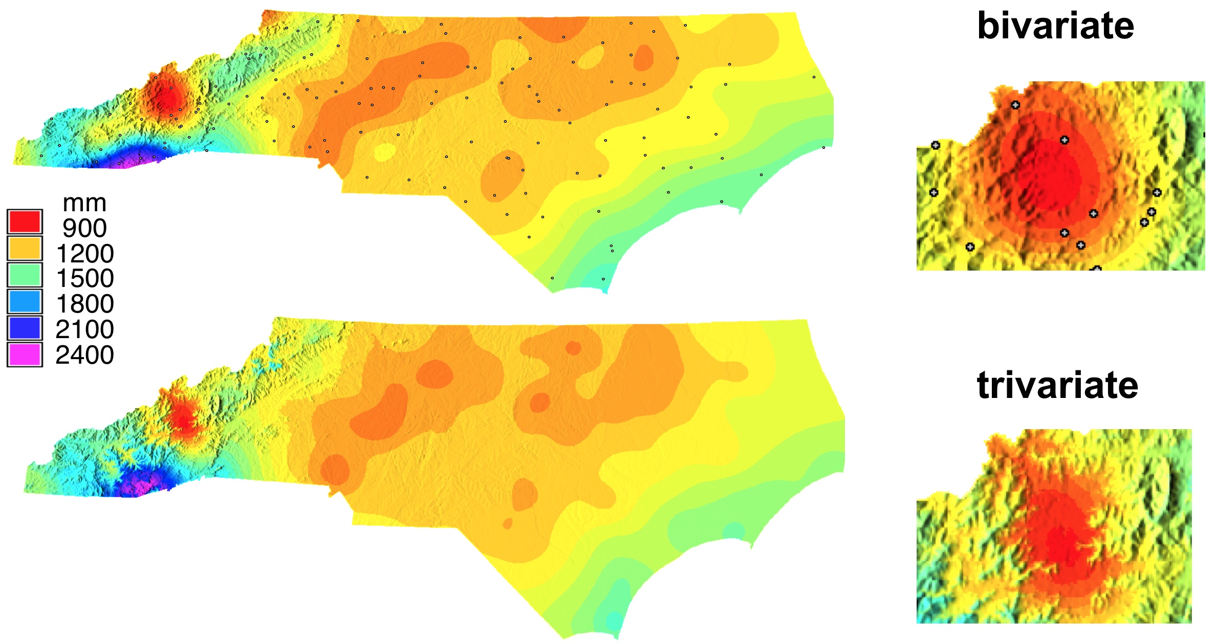
If sufficient data are available, the method captures increase of precipitation with elevation around Asheville and decrease of precipitation with elevation on the border with SC