# Ask GRASS GIS where its Python packages are.
sys.path.append(
    subprocess.check_output(["grass", "--config", "python_path"], text=True).strip()
)

# Import the GRASS GIS packages we need.
import grass.script as gs

# Import GRASS Jupyter
import grass.jupyter as gjSensitivity Analysis
Purpose
SIMWE (r.sim.water) solves the shallow-water flow equations with a Monte Carlo path sampling method, so its accuracy and cost depend on choices the user makes before the first walker moves: the spatial resolution of the DEM and the number of particles that sample the flow field. Running SIMWE with a high-resolution DEM and high particle density is computationally demanding. However, without a quantified understanding of how reducing spatial scale or particle density changes the results, it is difficult to optimize the trade-off between accuracy and runtime.
This notebook analyzes a factorial screening experiment across five physiographically distinct study areas: 4 spatial resolutions (1, 3, 10, and 30 m) x 4 particle-density scalars (0.25, 0.5, 1, and 2 walkers per cell) x 10 random seeds, or 160 SIMWE runs per site and 800 runs total (scripts/sensitivity.py, mapset sensitivity_7). Each run simulates a uniform 50 mm/hr rainfall with zero infiltration and Manning’s n of 0.1 for 120 one-minute iterations, writing depth and discharge every 10 minutes. We record the compute time of every run and derive spatial statistics of the seed-composited depth surfaces at each output step.
A scope note on the word “sensitivity”: this is a screening study of computational cost and Monte Carlo output variability, not a variance-based sensitivity analysis. No Sobol or Morris indices are computed here, and the physical parameters (rainfall, infiltration, Manning’s n) are held fixed. The commented SALib import below marks where that future work will attach; the accompanying manuscript’s discussion outlines the plan.
Experimental Design
The Site class below encapsulates the per-site analysis. A few conventions matter for everything that follows:
- Walker count. For each combination of resolution and density scalar, the number of particles is \(P = C \cdot S\), where \(C\) is the number of non-null cells in the simulation domain and \(S\) is the particle-density scalar. \(P\) is clamped to the range \([100, 7{,}000{,}000]\), so the smallest coarse-resolution runs are not at their nominal density.
- Simulation domain. At each resolution the DEM is resampled with bilinear interpolation, then
r.watershedextracts basins with a 30,000-cell accumulation threshold and the largest basin becomes the mask and region for the runs. Because the threshold is a cell count, the physical basin area grows with cell size (i.e., a 30,000-cell threshold is 0.03 km2 at 1 m but 27 km2 at 30 m), which is worth keeping in mind when comparing across resolutions. - Seed compositing. The 10 seeded runs of each configuration are composited per output step with
r.series(average, median, minimum, maximum, stddev, and range). Thestat_typecolumn that appears throughout the results refers to this across-seed composite method, not a statistic of the time series. - Terrain ruggedness. Each site’s Area Ruggedness Scale (ARS) is the mean Terrain Ruggedness Index (
r.tri, 13-cell moving window) over the study area, computed on the resampled DEM.
Study Areas
The five study areas span two orders of magnitude in terrain ruggedness, from the internally drained playas of the Texas High Plains to the steep forested headwater catchments of the southern Blue Ridge. That spread is deliberate: the slope and complexity of the terrain shape how sensitive the model is to particle density and resolution, so the same factorial design is repeated at every site.
| Site | State | Native res. | Area (km2) | ARS |
|---|---|---|---|---|
| tx069-playas | Texas | 8 m | 324.74 | 0.07 |
| clay-center | Kansas | 3 m | 1.53 | 0.13 |
| SJER | California | 1 m | 0.3 | 0.14 |
| SFREC | California | 1 m | 0.38 | 0.37 |
| coweeta | North Carolina | 10 m | 57.17 | 5.5 |
Site descriptions and full terrain summaries are in the per-site reports.
Data Assembly
Two derived tables drive the analysis. Both are expensive to build (the assembly cells re-run GRASS statistics over all 800 simulations), so they are marked eval: false and the executed cells below read the committed CSVs from output/combined_stats/ instead.
The first table, combined_analysis_7.csv (5,052 rows), combines the output of r.univar -e for each seed-composited depth raster into a single dataframe: one row per site x resolution x scalar x composite method (stat_type) x output step (minute), carrying the spatial statistics (min, max, mean, stddev, quartiles), the mean run time and particle count for that configuration, and the site’s ARS.
results_df = pd.read_csv(os.path.join("output", "combined_stats", 'combined_analysis_7.csv'))
results_df.info()
<class 'pandas.DataFrame'>
RangeIndex: 5052 entries, 0 to 5051
Data columns (total 26 columns):
# Column Non-Null Count Dtype
--- ------ -------------- -----
0 Unnamed: 0 5052 non-null int64
1 n 5052 non-null int64
2 null_cells 5052 non-null int64
3 cells 5052 non-null int64
4 min 5052 non-null float64
5 max 5052 non-null float64
6 range 5052 non-null float64
7 mean 5052 non-null float64
8 mean_of_abs 5052 non-null float64
9 stddev 5052 non-null float64
10 variance 5052 non-null float64
11 coeff_var 5048 non-null float64
12 sum 5052 non-null float64
13 first_quartile 5052 non-null float64
14 median 5052 non-null float64
15 third_quartile 5052 non-null float64
16 percentiles 5052 non-null str
17 run_time 5052 non-null float64
18 particles 5052 non-null float64
19 area_km2 5052 non-null float64
20 resolution 5052 non-null int64
21 scalar 5052 non-null int64
22 minute 5052 non-null int64
23 stat_type 5052 non-null str
24 ars 5004 non-null float64
25 Location 5052 non-null str
dtypes: float64(16), int64(7), str(3)
memory usage: 1.0 MBThe second table, combined_simulations_7.csv (8,346 rows), extracts the history that r.sim.water writes into each output raster’s metadata: the initialized walker count (init.walk), maximum and remaining walkers, mean flow velocity, time step, per-run compute time, and per-map min/max depth. One row per individual run x output step, so this table preserves the seed-to-seed variation that the composited table averages away.
model_runs_df = pd.read_csv(os.path.join("output", "combined_stats", 'combined_simulations_7.csv'))
model_runs_df.info()
<class 'pandas.DataFrame'>
RangeIndex: 8346 entries, 0 to 8345
Data columns (total 25 columns):
# Column Non-Null Count Dtype
--- ------ -------------- -----
0 Unnamed: 0 8346 non-null int64
1 init.walk 8346 non-null int64
2 maxwalk 8346 non-null int64
3 remaining walkers 8346 non-null int64
4 duration (sec.) 8346 non-null int64
5 mean man 8346 non-null float64
6 mean infil 8346 non-null float64
7 Location 8346 non-null str
8 map_name 8346 non-null str
9 Cells 8346 non-null int64
10 Min Depth (m) 8346 non-null float64
11 Max Depth (m) 8346 non-null float64
12 Seed 8346 non-null int64
13 Resolution (m) 8346 non-null int64
14 scalar_str 8346 non-null int64
15 Particle Scalar 8346 non-null float64
16 Number of iterations (cells) 8346 non-null int64
17 Mean flow velocity (m/s) 8346 non-null float64
18 Time Step (s) 8346 non-null float64
19 Time at Step (s) 8346 non-null float64
20 Time at Step (min) 8346 non-null float64
21 Mean Source Rate (Rain Fall Excess) (m/s) 8346 non-null float64
22 Compute Time (s) 8346 non-null float64
23 particles 8346 non-null float64
24 Particle Density 8346 non-null float64
dtypes: float64(13), int64(10), str(2)
memory usage: 1.6 MBsns.pairplot(model_runs_df, hue="Resolution (m)", kind="scatter")sns.pairplot(model_runs_df, hue="Location", kind="scatter")The composited table is grouped by resolution, scalar, site, composite method, and output step, averaging the numeric columns, then log-transformed copies of particles, run time, and ARS are added for the scaling plots below.
grouped_results_df = (results_df.groupby(by=['resolution', 'scalar', 'Location', 'stat_type', 'minute'])
        .agg({
            'run_time': 'mean',
            'particles': 'mean',
            'cells': 'mean',
            # 'area_km2': 'max',
            # 'p_density': 'max',
            # "minute": "mean",
            'mean': "mean",
            'ars': "mean",
            # "std": "mean",
            "max": "mean",
            "min": "mean",
            "stddev": "mean"
        })
        .reset_index()
)

grouped_results_df['log10(particles)'] = np.log10(grouped_results_df['particles'])
grouped_results_df['log10(run_time)'] = np.log10(grouped_results_df['run_time'])
grouped_results_df['log10(ars)'] = np.log10(grouped_results_df['ars'])
grouped_results_df['run_time_min'] = grouped_results_df['run_time'] / 60.0
grouped_results_df.head()| resolution | scalar | Location | stat_type | minute | run_time | particles | cells | mean | ars | max | min | stddev | log10(particles) | log10(run_time) | log10(ars) | run_time_min | |
|---|---|---|---|---|---|---|---|---|---|---|---|---|---|---|---|---|---|
| 0 | 1 | 1 | SFREC | average | 10 | 2780.749446 | 363592.0 | 491046.0 | 0.011785 | 0.960214 | 1.383436 | 0.000253 | 0.033582 | 5.560614 | 3.444162 | -0.017632 | 46.345824 |
| 1 | 1 | 1 | SFREC | average | 20 | 2780.749446 | 363592.0 | 491046.0 | 0.013080 | 0.960214 | 2.766822 | 0.000253 | 0.059275 | 5.560614 | 3.444162 | -0.017632 | 46.345824 |
| 2 | 1 | 1 | SFREC | average | 30 | 2780.749446 | 363592.0 | 491046.0 | 0.014045 | 0.960214 | 3.785676 | 0.000253 | 0.079292 | 5.560614 | 3.444162 | -0.017632 | 46.345824 |
| 3 | 1 | 1 | SFREC | average | 40 | 2780.749446 | 363592.0 | 491046.0 | 0.014865 | 0.960214 | 4.645530 | 0.000253 | 0.096456 | 5.560614 | 3.444162 | -0.017632 | 46.345824 |
| 4 | 1 | 1 | SFREC | average | 50 | 2780.749446 | 363592.0 | 491046.0 | 0.015598 | 0.960214 | 5.409575 | 0.000253 | 0.111816 | 5.560614 | 3.444162 | -0.017632 | 46.345824 |
model_runs_df.info()

# grouped_results_df['log10(particles)'] = np.log10(grouped_results_df['particles'])
model_runs_df['log10(Compute Time (s))'] = np.log10(model_runs_df['Compute Time (s)'])
# grouped_results_df['run_time_min'] = grouped_results_df['run_time'] / 60.0
# grouped_results_df.head()
<class 'pandas.DataFrame'>
RangeIndex: 8346 entries, 0 to 8345
Data columns (total 25 columns):
# Column Non-Null Count Dtype
--- ------ -------------- -----
0 Unnamed: 0 8346 non-null int64
1 init.walk 8346 non-null int64
2 maxwalk 8346 non-null int64
3 remaining walkers 8346 non-null int64
4 duration (sec.) 8346 non-null int64
5 mean man 8346 non-null float64
6 mean infil 8346 non-null float64
7 Location 8346 non-null str
8 map_name 8346 non-null str
9 Cells 8346 non-null int64
10 Min Depth (m) 8346 non-null float64
11 Max Depth (m) 8346 non-null float64
12 Seed 8346 non-null int64
13 Resolution (m) 8346 non-null int64
14 scalar_str 8346 non-null int64
15 Particle Scalar 8346 non-null float64
16 Number of iterations (cells) 8346 non-null int64
17 Mean flow velocity (m/s) 8346 non-null float64
18 Time Step (s) 8346 non-null float64
19 Time at Step (s) 8346 non-null float64
20 Time at Step (min) 8346 non-null float64
21 Mean Source Rate (Rain Fall Excess) (m/s) 8346 non-null float64
22 Compute Time (s) 8346 non-null float64
23 particles 8346 non-null float64
24 Particle Density 8346 non-null float64
dtypes: float64(13), int64(10), str(2)
memory usage: 1.6 MBResults
Computational Cost
The first figure is a diagnostic rather than a result: it compares the walker count we requested (nwalkers, x-axis) against the count SIMWE actually initialized (init.walk, y-axis). The relationship should be the identity line; departures at the low end are the 100-walker minimum clamp firing on the coarse-resolution runs (e.g., SJER at 30 m with a 0.25 scalar requests 81 walkers and gets 100).
sns.set_theme(style="darkgrid")
sns.set_context("talk")
sns.color_palette("crest", as_cmap=True)
fig, ax = plt.subplots(figsize=(12, 8))
sns.lineplot(
    data=model_runs_df,
    x="particles",
    y="init.walk",
    hue="Location",
    style="Resolution (m)",
    # size="scalar",
    err_style="bars",
    # errorbar=("se", 2),
    palette="magma",
    markers=True,
    alpha=0.75,
    errorbar=('ci', 95),
)
sns.move_legend(ax, "upper left", bbox_to_anchor=(1, 1))
plt.xlabel("nwalk", fontsize=26)
plt.ylabel("init.walk", fontsize=26)
# plt.title("Resolution vs Run Time")
plt.savefig(f"../output/nwalk_init_walk.png")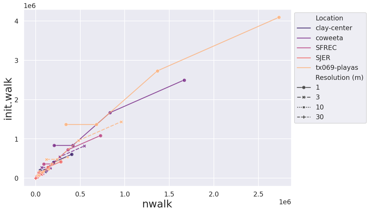
Compute time is driven primarily by the total number of particles, and since particles scale with cell count, spatial resolution dominates. Moving from 30 m to 1 m raises the cell count by nearly three orders of magnitude, and the log-scale compute times below track that increase across every site.
sns.set_theme(style="darkgrid")
sns.set_context("talk")
sns.color_palette("crest", as_cmap=True)
fig, ax = plt.subplots(figsize=(12, 8))
sns.lineplot(
    data=model_runs_df,
    x="Resolution (m)",
    y="log10(Compute Time (s))",
    hue="Location",
    style="Particle Density",
    # size="scalar",
    err_style="bars",
    # errorbar=("se", 2),
    palette="magma",
    markers=True,
    alpha=0.75,
    errorbar=('ci', 95),
)
sns.move_legend(ax, "upper left", bbox_to_anchor=(1, 1))
plt.xlabel("Resolution (m)", fontsize=26)
plt.ylabel("log10(Compute Time (s))", fontsize=26)
# plt.title("Resolution vs Run Time")
plt.savefig(f"../output/compute_time_by_resolution.png")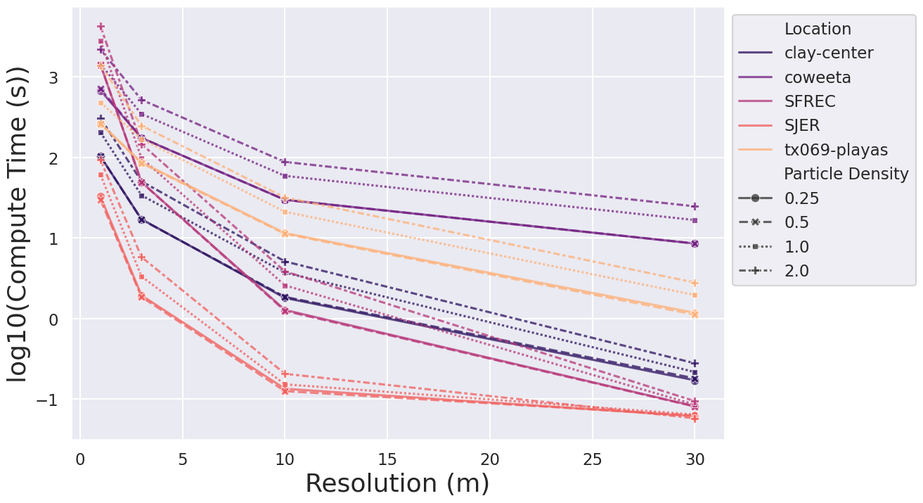
Particle density matters much less than resolution. Doubling the density scalar roughly doubles the walkers, but the compute-time curves below are nearly flat compared to the resolution effect above, which is the practical takeaway for users: reducing resolution buys far more runtime than reducing density, at a correspondingly larger cost in spatial detail.
sns.set_theme(style="darkgrid")
sns.set_context("talk")
sns.color_palette("crest", as_cmap=True)
fig, ax = plt.subplots(figsize=(12, 8))
# model_runs_df['log10(run_time)'] = np.log10(model_runs_df['run_time'])
sns.lineplot(
    data=model_runs_df,
    x="Particle Density",
    y="log10(Compute Time (s))",
    hue="Location",
    style="Resolution (m)",
    # size="AR",
    err_style="bars",
    # errorbar=("se", 2),
    palette="magma",
    markers=True,
    alpha=0.75,
    errorbar=('ci', 95),
)
sns.move_legend(ax, "upper left", bbox_to_anchor=(1, 1))
# g = sns.JointGrid(data=model_runs_df, x="Particle Density", y="log10(run_time)", space=0)
# g.plot_joint(sns.kdeplot,
#              fill=True, clip=((0, 3), (-2.0, 3.0)),
#              thresh=0, levels=100, cmap="rocket")
# g.plot_marginals(sns.histplot, palette="rocket", hue="Location", alpha=1, bins=25, data=model_runs_df)
plt.xticks([0.25, 0.5, 0.75, 1, 1.25, 1.5, 1.75, 2])
plt.xlabel("Particle Density", fontsize=26)
plt.ylabel("log10(Compute Time (s))", fontsize=26)
plt.savefig(f"../output/compute_time_by_particle_density.png")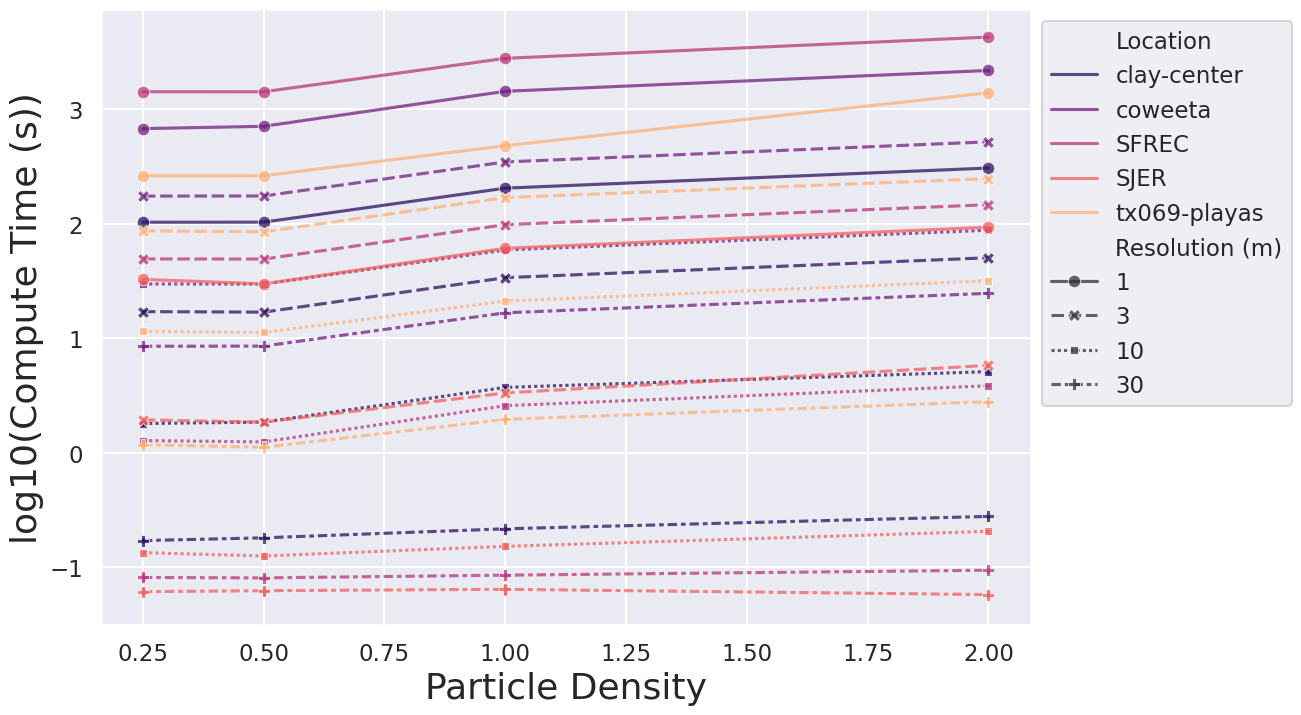
Water Depth and Velocity
The next figures shift from cost to output. Max Depth (m) here is the per-run raster maximum reported in each output map’s history (i.e., a per-seed value, not the across-seed composite). As resolution decreases, cells grow and the same water volume spreads over fewer, larger cells, so simulated depths increase; coarser runs also approach steady state sooner.
sns.set_theme(style="darkgrid")
sns.set_context("talk")
sns.color_palette("crest", as_cmap=True)
fig, ax = plt.subplots(figsize=(12, 8))
sns.lineplot(
    data=model_runs_df,
    x="Time at Step (min)",
    y="Max Depth (m)",
    hue="Location",
    style="Resolution (m)",
    size="Resolution (m)",
    err_style="bars",
    # errorbar=("se", 2),
    palette="magma",
    markers=True,
    alpha=0.75,
    errorbar=('ci', 95),
)
sns.move_legend(ax, "upper left", bbox_to_anchor=(1, 1))
plt.xlabel("Time at Step (min)", fontsize=26)
plt.ylabel("Max Depth (m)", fontsize=26)
# plt.title("Simulation Time Step vs Max Water Depth")
plt.savefig(f"../output/simulated_timestep_max_water_depth.png")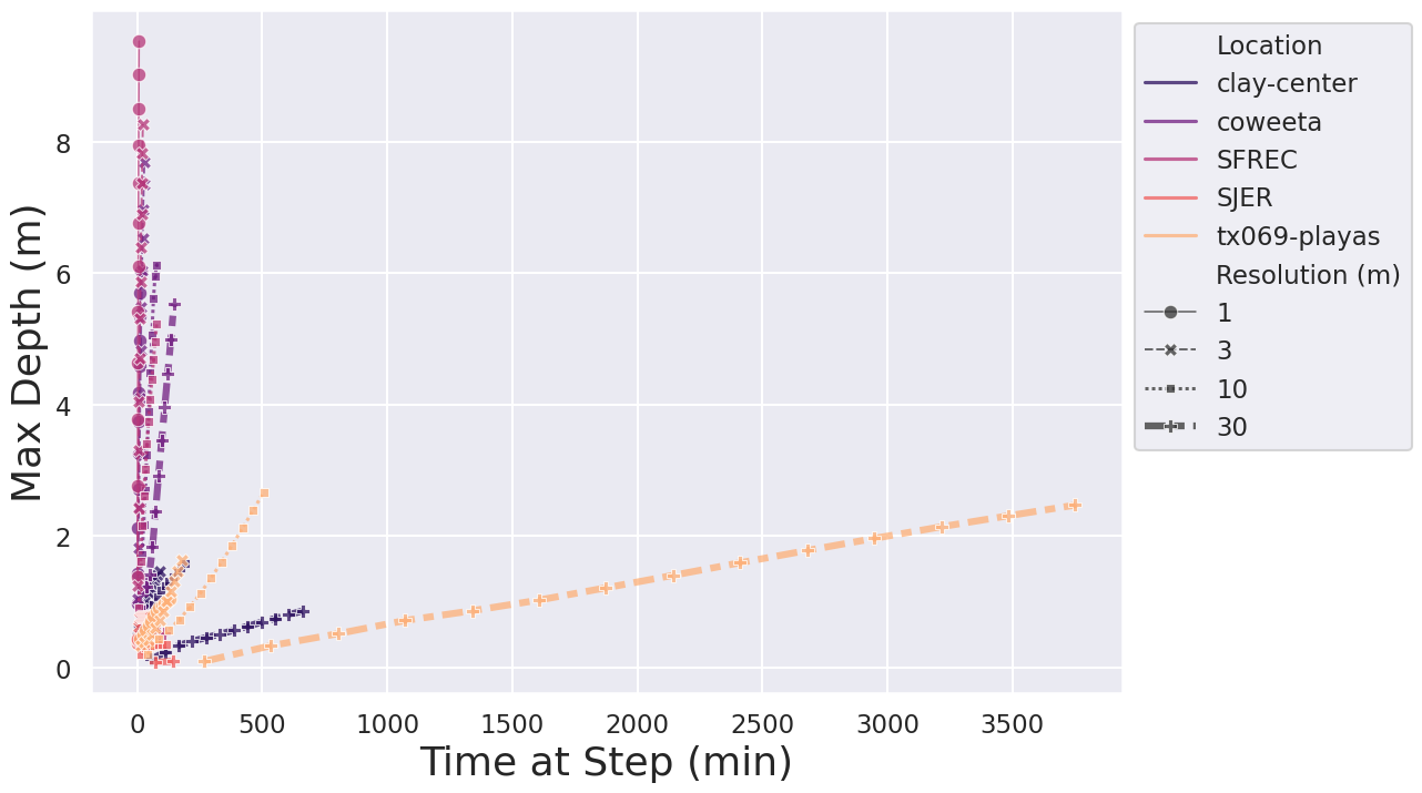
Mean flow velocity by output step, faceted by particle density (columns) and resolution (rows). The strip plots show the per-run spread; velocity stabilizes within the first few output steps at every density, another indication that density mainly affects the smoothness of the pattern rather than the bulk hydraulics.
sns.set_theme(style="darkgrid")
sns.set_context("paper")
sns.color_palette("crest", as_cmap=True)
g = sns.catplot(
    data=model_runs_df,
    x="Time at Step (min)",
    y="Mean flow velocity (m/s)",
    hue="Location",
    col="Particle Density",
    row="Resolution (m)",
    palette="YlGnBu_d",
    sharex=False,
    sharey=False,
    # errorbar="se",
    kind="strip",
    height=6, aspect=.75,
)
g.despine(left=True)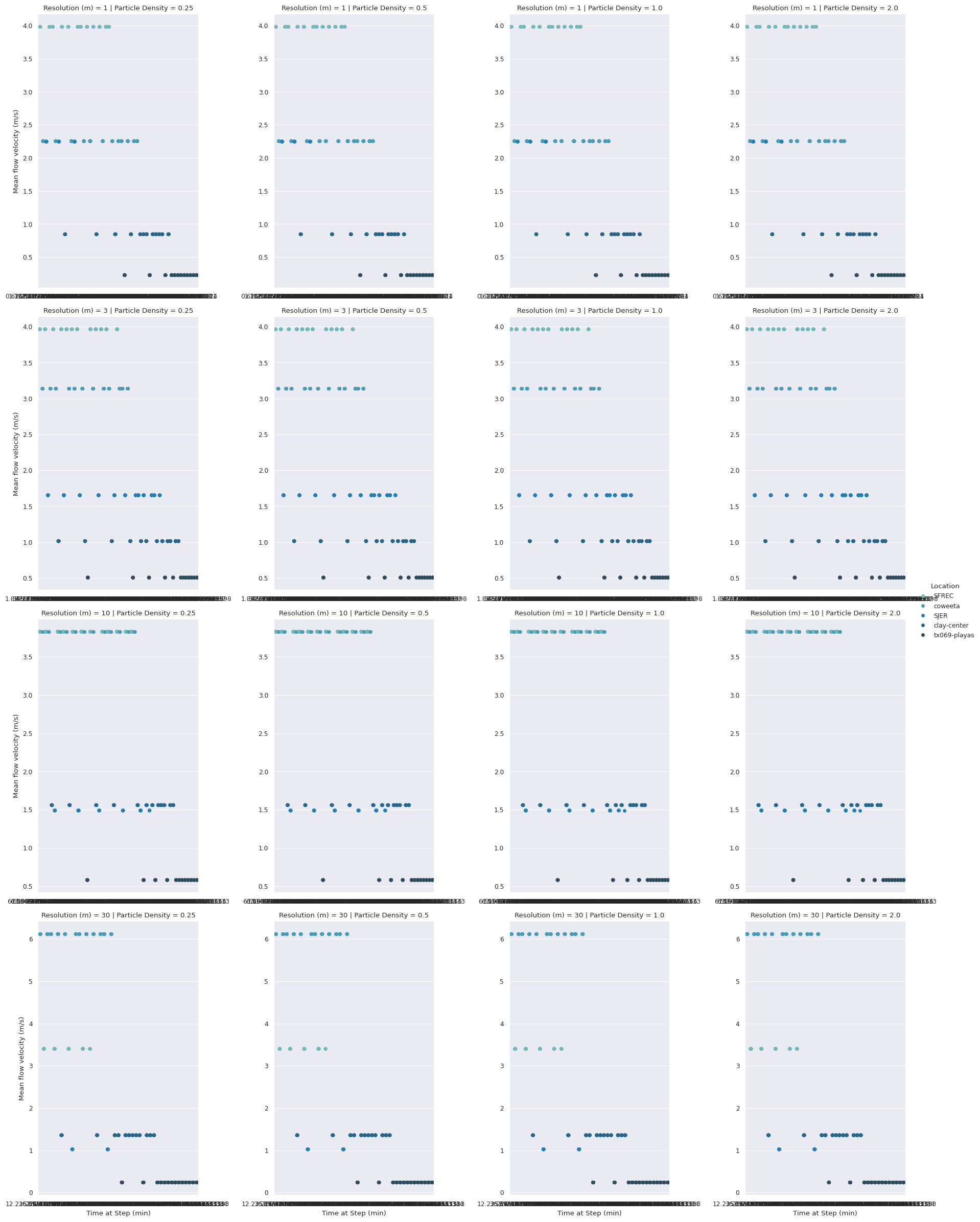
The remaining cells in this section are exploratory variants of the plots above, built from the ungrouped composite table. They are not executed in the rendered page (eval: false is the document default); the code is kept for reference.
sns.set_theme(style="darkgrid")
sns.set_context("paper")
sns.color_palette("crest", as_cmap=True)
fig, ax = plt.subplots(figsize=(12, 8))
sns.lineplot(
    data=results_df,
    x="resolution",
    y="run_time",
    hue="Location",
    style="scalar",
    # size="scalar",
    err_style="bars", errorbar=("se", 2),
    palette="magma",
    markers=True,
    alpha=0.75,
    # errorbar=('ci', 95),
)
plt.title("Resolution vs Run Time")sns.set_theme(style="darkgrid")
sns.set_context("paper")
sns.color_palette("crest", as_cmap=True)
fig, ax = plt.subplots(figsize=(12, 8))
sns.lineplot(
data=results_df,
x="scalar",
y="run_time",
hue="Location",
style="resolution",
# size="scalar",
err_style="bars", #errorbar=("se", 2),
palette="magma",
markers=True,
alpha=0.75,
errorbar=('ci', 95),
)
plt.title("Particles Density vs Run Time")
# plt.savefig(f"../output/agu2024_particles_run_time.png")sns.set_theme(style="darkgrid")
sns.set_context("paper")
sns.color_palette("crest", as_cmap=True)
# fig, ax = plt.subplots(figsize=(12, 8))
sns.relplot(
data=results_df, x="resolution", y="run_time",
col="Location",
hue="Location", style="scalar",
kind="line"
)
# sns.lineplot(
# data=grouped_results_df,
# x="scalar",
# y="run_time",
# hue="site_name",
# style="resolution",
# # size="scalar",
# err_style="bars", #errorbar=("se", 2),
# palette="magma",
# markers=True,
# alpha=0.75,
# errorbar=('ci', 95),
# )
plt.title("Particles Density vs Run Time")Text(0.5, 1.0, 'Particles Density vs Run Time')
sns.relplot(
    data=results_df, x="particles", y="run_time",
    col="Location",
    hue="Location", style="scalar",
    kind="line"
)
Terrain Ruggedness
Terrain relief also shapes compute cost. Sites with higher ARS drain water off the surface faster, so fewer walkers persist through the later iterations and runs finish sooner than at flatter sites with comparable cell counts. The cells below explore that relationship (run time against ARS, raw and log-transformed). Two caveats when reading them: ARS is computed with a fixed 13-cell window, so its physical footprint grows with cell size, and the simulation domain area also changes with resolution, so the ARS axis mixes terrain signal with scale effects.
sns.set_theme(style="darkgrid")
sns.set_context("talk")
sns.color_palette("crest", as_cmap=True)
fig, ax = plt.subplots(figsize=(12, 8))
# sns.lineplot(
#     data=grouped_results_df.query("stat_type == 'average'"),
#     # x="p_density",
#     x="ars",
#     y="max",
#     # y="run_time_min",
#     hue="site_name",
#     size="scalar",
#     palette="crest_r",
#     markers=True,
#     # style='resolution',
#     alpha=0.75,
#     errorbar=('ci', 95)
# )


# ax2 = plt.twinx()

sns.lineplot(
    data=grouped_results_df.query("stat_type == 'average'"),
    # x="p_density",
    x="ars",
    y="run_time",
    # y="run_time_min",
    hue="Location",
    # size="resolution",
    palette="magma",
    markers=True,
    style='resolution',
    alpha=0.75,
    errorbar=('ci', 95),
    # ax=ax2
)
plt.xlabel("ARS", fontsize=26)
plt.ylabel("Compute Time (s)", fontsize=26)
# plt.title("Run time vs. ARS", fontsize=32)
# plt.legend(title="Particle Density", fontsize=18)
sns.move_legend(ax, "upper left", bbox_to_anchor=(1.25,1))
# sns.move_legend(ax2, "upper left", bbox_to_anchor=(1.25,0.25))
# ax2.set_ylabel("Resolution (m)", fontsize=26)

# plt.savefig(os.path.join("../output", site, mapset, f'{site}_run_time_res_line_plot.png'))

plt.savefig(f"../output/sensitivity7_run_time_ars_plot.png")
plt.show()
# g = sns.JointGrid(data=grouped_results_df.query("stat_type == 'average'"), x="ars", y="run_time", space=0)
# g.plot_joint(sns.kdeplot,
# fill=True, clip=((0, 3), (0, 200)),
# thresh=0, levels=100, cmap="rocket")
# g.plot_marginals(sns.histplot, color="#03051A", alpha=1, bins=25)
# Plot sepal width as a function of sepal_length across days
g = sns.lmplot(
data=grouped_results_df.query("stat_type == 'average'"),
x="ars", y="run_time", hue="Location",
height=5
)
# Use more informative axis labels than are provided by default
g.set_axis_labels("ARS", "Compute Time (Sec)")sns.set_theme(style="darkgrid")
sns.set_context("talk")
sns.color_palette("crest", as_cmap=True)
fig, ax = plt.subplots(figsize=(12, 8))
sns.despine(fig, left=True, bottom=True)
# scalar_ranking = ["I1", "SI2", "SI1", "VS2", "VS1", "VVS2", "VVS1", "IF"]
sns.scatterplot(
# x="ars",
# y="run_time",
x="log10(ars)",
y="log10(run_time)",
hue="Location", size="resolution",
style="scalar",
# palette="ch:r=-.2,d=.3_r",
palette="magma",
# hue_order=clarity_ranking,
sizes=(10, 50), linewidth=0,
data=grouped_results_df.query("stat_type == 'average'"), ax=ax
)
# sns.regplot(
# data=grouped_results_df.query("stat_type == 'average' and Location == 'clay-center'"),
# x="ars",
# y="run_time",
# order=2,
# color="black",
# ci=95,
# scatter=False,
# line_kws=dict(linewidth=1, linestyle="--"),
# )
# sns.regplot(
# data=grouped_results_df.query("stat_type == 'average' and Location == 'coweeta'"),
# x="ars",
# y="run_time",
# order=2,
# color="black",
# ci=95,
# scatter=False,
# line_kws=dict(linewidth=1, linestyle="--"),
# )
# sns.regplot(
# data=grouped_results_df.query("stat_type == 'average' and Location == 'SJER'"),
# x="ars",
# y="run_time",
# order=2,
# color="black",
# ci=95,
# scatter=False,
# line_kws=dict(linewidth=1, linestyle="--"),
# )
sns.move_legend(ax, "upper left", bbox_to_anchor=(1, 1))
plt.xlabel("ARS", fontsize=26)
plt.ylabel("log10(Compute Time (Sec))", fontsize=26)
plt.savefig(f"../output/sensitivity7_ars_run_time_loc_res_scalar_plot.png")sns.set_theme(style="darkgrid")
sns.set_context("talk")
sns.color_palette("crest", as_cmap=True)
fig, ax = plt.subplots(figsize=(12, 8))
sns.lineplot(
data=grouped_results_df,
x="log10(particles)",
y="log10(run_time)",
hue="Location",
# size="resolution",
style="resolution",
# weights="error",
palette="magma",
markers=True,
alpha=0.75,
errorbar=('ci', 95),
)
plt.xlabel("log10(Particles)", fontsize=26)
plt.ylabel("log10(Compute Time (s))", fontsize=26)
sns.move_legend(ax, "upper left", bbox_to_anchor=(1, 1))
# plt.title("Particles vs Run Time")
# plt.savefig(f"../output/agu2024_particles_run_time.png")
plt.savefig(f"../output/particles_run_time.png")sns.set_theme(style="darkgrid")
sns.set_context("talk")
sns.color_palette("crest", as_cmap=True)
fig, ax = plt.subplots(figsize=(12, 8))
sns.lineplot(
data=grouped_results_df,
x="cells",
y="log10(particles)",
hue="Location",
style="scalar",
palette="magma",
markers=True,
alpha=0.75,
errorbar=('ci', 95),
)
sns.move_legend(ax, "upper left", bbox_to_anchor=(1, 1))
plt.title("Particles vs Resolution")
# plt.savefig(f"../output/agu2024_particles_resolution.png")sns.set_theme(style="darkgrid")
sns.set_context("talk")
sns.color_palette("crest", as_cmap=True)
fig, ax = plt.subplots(figsize=(12, 8))
sns.lineplot(
data=grouped_results_df.query("stat_type == 'average'"),
x="log10(particles)",
y="log10(run_time)",
hue="cells",
style="Location",
# size="scalar",
palette="magma_r",
markers=True,
alpha=0.75,
errorbar=('ci', 95),
)
sns.move_legend(ax, "upper left", bbox_to_anchor=(1, 1))
plt.xlabel("log10(Particles)", fontsize=26)
plt.ylabel("log10(Compute Time (s))", fontsize=26)
# plt.title("ARS vs log10(Run Time)")
plt.savefig(f"../output/agu2024_ars_run_time.png")sns.set_theme(style="darkgrid")
sns.set_context("talk")
sns.color_palette("crest", as_cmap=True)
fig, ax = plt.subplots(figsize=(12, 8))
sns.lineplot(
data=grouped_results_df.query("stat_type == 'average'"),
x="log10(particles)",
y="max",
hue="Location",
# style="minute",
palette="magma_r",
markers=True,
alpha=0.75,
errorbar=('ci', 95),
)
sns.move_legend(ax, "upper left", bbox_to_anchor=(1, 1))
plt.title("log10(particles) by Max Depth")Depth by Output Step
The final series tracks the seed-composited depth statistics through the 120-minute event. A note on semantics that applies to all four plots: the y-axis is always the spatial mean of the across-seed composite named in the query, so “the mean of the maximum composite” is the spatial average of the 10-seed maximum raster, not the maximum depth. Coarser resolutions plot deeper and flatten earlier, the steady-state result from the manuscript; the stddev composite shows where the 10 seeds disagree, which is the Monte Carlo noise floor of the method.
sns.set_theme(style="darkgrid")
sns.set_context("talk")
sns.color_palette("crest", as_cmap=True)
fig, ax = plt.subplots(figsize=(12, 8))
sns.lineplot(
    data=grouped_results_df.query("stat_type == 'average'"),
    x=grouped_results_df.query("stat_type == 'average'")["minute"].astype(int),
    y="mean",
    hue="Location",
    style="resolution",
    size="resolution",
    palette="magma",
    markers=True,
    alpha=0.75,
    errorbar=('ci', 95),
)
# plt.title("Mean Depth by Output Step")
plt.xlabel("Output Step (Minutes)", fontsize=26)
plt.ylabel("Mean Depth (m)", fontsize=26)
sns.move_legend(ax, "upper left", bbox_to_anchor=(1, 1))

plt.savefig(f"../output/agu2024_minute_mean_resolution.png")sns.set_theme(style="darkgrid")
sns.set_context("talk")
sns.color_palette("crest", as_cmap=True)
fig, ax = plt.subplots(figsize=(12, 8))
sns.lineplot(
data=grouped_results_df.query("stat_type == 'maximum'"),
x=grouped_results_df.query("stat_type == 'maximum'")["minute"].astype(int),
y="mean",
hue="Location",
size="resolution",
style="resolution",
palette="magma",
markers=True,
alpha=0.75,
errorbar=('ci', 95),
)
plt.xlabel("Output Step (Minutes)", fontsize=26)
plt.ylabel("Maximum Depth (m)", fontsize=26)
sns.move_legend(ax, "upper left", bbox_to_anchor=(1, 1))
# plt.title("Maximum Depth by Output Step")
plt.savefig(f"../output/agu2024_minute_max_resolution.png")sns.set_theme(style="darkgrid")
sns.set_context("paper")
sns.color_palette("crest", as_cmap=True)
fig, ax = plt.subplots(figsize=(12, 8))
sns.lineplot(
data=grouped_results_df.query("stat_type == 'minimum'"),
x=grouped_results_df.query("stat_type == 'minimum'")["minute"].astype(int),
y="mean",
hue="Location",
style="resolution",
size="resolution",
palette="magma",
markers=True,
alpha=0.75,
errorbar=('ci', 95),
)
# plt.title("Min Depth by Time Step")
plt.xlabel("Output Step (Minutes)", fontsize=26)
plt.ylabel("Minimum Depth (m)", fontsize=26)
sns.move_legend(ax, "upper left", bbox_to_anchor=(1, 1))
plt.savefig(f"../output/agu2024_minute_min_resolution.png")sns.set_theme(style="darkgrid")
sns.set_context("talk")
sns.color_palette("crest", as_cmap=True)
fig, ax = plt.subplots(figsize=(12, 8))
sns.lineplot(
data=grouped_results_df.query("stat_type == 'stddev'"),
x=grouped_results_df.query("stat_type == 'stddev'")["minute"].astype(int),
y="mean",
hue="Location",
style="resolution",
size="resolution",
palette="magma",
markers=True,
alpha=0.75,
errorbar=('ci', 95),
)
plt.title("Stddev Depth by Time Step")
sns.move_legend(ax, "upper left", bbox_to_anchor=(1, 1))
plt.savefig(f"../output/agu2024_minute_std_resolution.png")sns.set_theme(style="darkgrid")
sns.set_context("paper")
sns.color_palette("crest", as_cmap=True)
fig, ax = plt.subplots(figsize=(12, 8))
sns.lineplot(
data=grouped_results_df.query("stat_type == 'average' & Location == 'clay-center'"),
x=grouped_results_df.query("stat_type == 'average' & Location == 'clay-center'")["minute"].astype(int),
y="mean",
hue="resolution",
# style="resolution",
size="scalar",
palette="summer",
markers=True,
alpha=0.75,
errorbar=('ci', 95),
)
sns.lineplot(
data=grouped_results_df.query("stat_type == 'average' & Location == 'SJER'"),
x=grouped_results_df.query("stat_type == 'average' & Location == 'SJER'")["minute"].astype(int),
y="mean",
hue="resolution",
# style="scalar",
size="scalar",
palette="cool",
markers=True,
alpha=0.75,
errorbar=('ci', 95),
)
plt.title("Mean Depth by Time Step, Clay Center and SJER")
plt.savefig(f"../output/agu2024_minute_average_scalar.png")Discussion and Next Steps
Three results carry the practical weight of this analysis. First, compute time is governed by the total particle count, so spatial resolution, which sets the cell count, dominates runtime; particle density is a second-order cost. Second, coarser resolutions systematically produce deeper water and reach steady state sooner, so resolution is not a neutral performance knob: it changes the answer, not just the wait. Third, terrain matters, with higher-ARS sites draining faster and costing less compute per cell than flat sites like the Texas playas, where water lingers in depressions for the full event.
However, several limitations shape how far these numbers travel. The basin extraction threshold is a fixed cell count (30,000), so the physical simulation domain grows with cell size, up to a 68x area difference within a single site across the resolution range; the resolution effect and the domain-size effect are therefore confounded in the compute-time figures. The final output steps are irregular at some sites (coarse grids drain early and stop), so the late-time portions of the depth curves rest on fewer observations than the error bands suggest. Both issues are being addressed in the accompanying manuscript.
For the spatial, single-site view of the same seed-to-seed variability, see Model Run Variability, which maps where the Gaussian path-sampling noise concentrates. The per-site reports carry the basin-extent overlap figures and seed-averaged depth maps for each study area.
This screening study is a first step. In future work, a more comprehensive global sensitivity analysis should include the physical parameters held fixed here (i.e., rainfall intensity, Manning’s coefficient, infiltration, and diffusivity), using the Sobol method via SALib to attribute output variance to individual parameters and their interactions.