Geospatial data acquisition

Helena Mitasova

GIS/MEA582 Geospatial Modeling and Analysis NCSU

Learning objectives

• Understand the diversity of geospatial data sources
• Classify modern mapping technologies
• Understand the concept of georeferenced data
• Explain priciples of coordinate reference systems (CRS)
• Define raster and vector data models
• Distinguish between continuous and discrete phenomena

Geospatial data acquisition

Current revolution in mapping technologies:

Continuous data collection anywhere by anyone

Professional mapping technologies

• passive and active aerial and satellite sensors
• ground-based sensors: (RTK)GPS, total station, lidar
• in situ sensors measuring environmental variables: air and water quality, river stages, soil moisture, ...

Emergence of autonomous platforms: air, ground, water

Remote sensing: passive

Numerous satellite and airborne platforms and sensors, for example:

• Landsat 1-9: landcover since 1972, 30m, multispectral
• Terra: MODIS temperature 250m; ASTER radiance, DEM
• SENTINEL 1-5P: landcover, temperature, ocean currents, atmosphere, multispectral
• PLANET: new generation of small satellites: 170 small satellites mapping Earth daily at 3m resolution

Learn in GIS512 Introduction to Environmental Remote Sensing

Remote sensing: active

Satellite and airborne platforms and sensors, examples:

• Shuttle Radar Topography Mission (SRTM) 2001: 30m resolution elevation for almost entire globe
• InSAR: high accuracy deformation mapping
• Lidar: airborne surveys - high resolution elevation data, including vegetation structure

See overview of Remote Sensors by NASA

Learn in GIS512 Introduction to Environmental Remote Sensing

Satellite Remote Sensing

SRTM and LANDSAT example for Panama:

Images and data by NASA and NCSU MEAS

Satellite Remote Sensing

PLANET images for Jockey's Ridge change between September 2017 and July 2018 mapped at 3m resolution:

Data by planet.com

Airborne Remote Sensing

Lidar and orthophoto example for NCSU fields - sub-meter resolution mapping:

Most current systems combine active and passive sensors

Airborne Remote Sensing

3D construction site mapping at cm resolution using small unmanned aerial system (drone)

Mapped in 2021 by William Reckling, NCSU graduate student
NCSU GeoForAll Lab 3D models from UAS on sketchfab,
learn in GIS584 Mapping and Analytics Using UAS

Ground-based passive

Airborne orthophoto compared with on-ground mobile 360 degree camera streetview

Credits: Orthphoto from NC One Map, Ground-based image from Google streetview

Ground-based active

Terrestrial lidar: monitoring eroding stream bank at mm resolutions

Credits: Photo and data by Nathan Lyons, NCSU graduate student, 3D model by Helena Mitasova

Non-traditional data sources

Widespread GPS enabled technology:

• smartphones, tablets (GPS and lidar)
• webcams (AMOS)
• mobile sensor networks : cars, bicycles, scooters
• smart devices (internet of things): trash cans, utilities

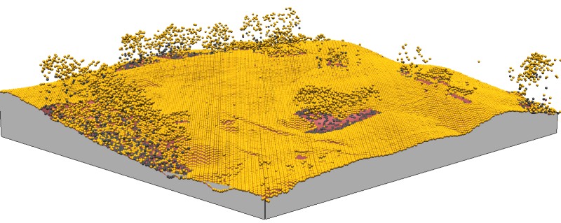
Time spent by a group of people along a guided tour, displayed over a lidar-based DSM, learn more in Mitas et al., 2020

From mapping to GIS

Acquired data are transformed into georeferenced, discrete representations of landscape features

• georeferencing (often in real-time using GPS)
• feature or theme extraction (e.g. image classification)
• building GIS data model representation
  (geometry, attributes, time)
• generating metadata

Georeferencing

Georeferenced data: location on Earth is represented in a Coordinate Referenced System (CRS)

• geodetic (geographic) coordinate system:
  geoid -- ellipsoid -- latitude/longitude

• projected reference systems:
  geoid -- ellipsoid -- developable surface -- plane -- x,y

Geodetic (Geographic) CRS

geoid -- ellipsoid -- latitude/longitude

• GPS, large regions, data exchange
• units: degree-minutes-seconds
• complex algorithms for distances, areas

Projected CRS

Projected reference systems (there are many):
geoid -- ellipsoid -- developable surface -- plane -- x,y

• developable surfaces: conic, cylindrical, azimuthal
• type of distortion: conformal, equidistant, equal area

Map projection transitions Cartographic projections by Furuti

National and state CRS

Defined by:

• Reference spheroid/geoid and datum:
  e.g. GRS80-NAD83, WGS84, NATR2022
• Projection and its parameters, e.g. :
  • Lambert Conformal Conic (LCC): states in US
  • Universal Transverse Mercator (UTM): USGS, military
  • Albers Equal Area (conic): USGS national map
• Vertical datum: e.g. NAVD88, NAPGD2022

NAD83 and NAVD88 to be replaced with North American Terrestrial Reference Frame (NATR2022) and North American-Pacific Geopotential Datum of 2022 (NAPGD2022)

CRS standards

CRS have standardized definition with assigned EPSG codes (initiated by European Petroleum Survey Group)

EPSG codes and CRS representation in many formats is avaiable at epsg.io or Spatial Reference website Example: EPSG:4326 WGS84 used in GPS

Transition to ISO 19111:2019 international standard notation in WKT:well known text (text markup language)

Popular Visualization CRS

World map in Pseudo Mercator with massive distortions farther from the equator, compared with Winkel-Tripel projection with more realistic representation

Although the EPSG committee stated that they will not devalue the EPSG dataset by including such inappropriate geodesy and cartography, Pseudo Mercator was eventually included as EPSG 3857 - it is not recommended for professional work

Coordinate transformations

Geospatial data often come in different CRS, e.g.:

• Federal agencies: Geodetic CRS (WGS84), Albers equal area, UTM
• State agencies: State Plane CRS
• Older data may have different datums (NAD27, NAD83)

Coordinate transformations

x,y -> longitude, latitude -> x’,y’

often performed on-fly, may be inaccurate and time consuming

• first reproject all data into a suitable common CRS
• then perform analysis and modeling

Geospatial data models

Mapped data, results of modeling or analysis are represented in GIS using

• raster (regular grid) data model
• vector (feature) data model
• specialized representations: meshes

Geospatial phenomena

• Continuous fields
  • elevation surfaces
  • temperature, precipitation
  • concentration of chemicals in soil or water bodies

• Discrete features: lines, points or areas with attributes
  • roads, buildings, cell towers
  • land use types, administrative units

• Some phenomena can be treated as both types
  • agricultural fields (crop type vs. crop height), soil properties
  • population densities

Continuous fields

• each point in space is assigned a distinct value, change in values between neighboring points is small
• mathematical representation: bi-variate or multi-variate continuous functions $w=f(x,y), w=f(x,y,z), w=f(x,y,z,t)$
• often represented by a raster data model
• vector model is also used: isolines, meshes, or points.

Discrete objects / features

• points, lines, or areas (polygons) with attributes
• represented by vector data model as geometry(shape) with attribute table
• raster representation is also used

Raster data model: 2D

• header: spatial extent and resolution, followed by matrix of values (INT, FP, DP),
• continuous field : value assigned to a grid point
• discrete object : category value assigned to pixel (area)

Raster data model: continuous fields

Raster data model: discrete features

Land use classes at 30m resolution, qualitative data

Raster data model: discrete features

Roads: Speed limits for roads and walking speed for off-road areas, 30m resolution, quantitative data

Raster data model: 3D hybrid

Cross-sections through 3D model of soil horizons

Raster data model: 3D grid

• header + 3D matrix of values, voxel model
• spatial extent N,S,E,W,Top, Bottom
• vertical resolution is usually much finer than horizontal
• often used for 3D continuous representation $w=f(x,y,z)$

Soil properties: Percent organic carbon, soil pH reaction

Vector data model

Abstract representation of complex features
school – point, road – centerline, park - polygon

• Geometry:
  • Points [x,y,(z)] represent point, line, or polygon(area) features
  • Set of points create elements of feature geometry: line: nodes, vertices; polygon: centroid, boundary
  • Geospatial Topology defines how the elements of feature geometry are interrelated and organized (don't confuse with topography!)
  • Topology ensures integrity of features and efficiency by defining shared coincident geometry (shared boundaries, nodes).

• Attributes are stored in data management systems

Vector data model geometry

Vector data model geometry

Elements: vertices(red), nodes(blue), centroids(green)

Polygons: vertices+nodes=boundaries, centroids

Vector data model examples

Geometry and attributes for point, line and polygon data:

Vector data: 3D models

Full 3D meshes: representation of structures

Common geospatial data formats

Format: specific implementation of data model,
open standard or proprietary

Raster

• GIS (ascii and binary): GeoTIFF, ArcGRID, GRASS, SURFER
• Imagery: MrSID, GeoTIFF, BIN, JPEG2000, IMG
• Graphics: GIF, JPG, PNG, Bitmap
• HDF, NetCDF

Vector

• GeoPackage exchange format, KML, Shape, ArcSDE, GML, MapInfo, TIGER
• PostGIS, OracleSpatial

Geospatial data format conversion

Format description is usually stored with data: automated format recognition and conversion

General library for geospatial raster and vector format conversions:
Geospatial Data Abstraction Library (GDAL/OGR)
gdal.org

given format - single abstract model - new format

GDAL includes command line utilities for data processing

Coupled with PROJ library it also provides coordinate system transformations

Summary

• we provided overview of modern technologies for geospatial data acquisition
• we explained the concept of coordinate reference systems and related standards
• we introduced raster and vector data models and showed how they are used to represent continuous and discrete geographic phenomena