Process-based water flow simulation
Helena Mitasova, Anna Petrasova, Vaclav Petras
GIS714 Geosimulations NCSU
Learning objectives
- surface water flow modeling components
- shallow water flow equations
- numerical methods, path sampling
- applications: surface runoff, dam breach
- visualization of surface water flow dynamics
Modeling components: overland flow
- Modeled quantity: water depth [m], discharge [m$^3$/s]
- Spatial and temporal scale: first order stream [1m resolution], single storm [minutes]
- Configuration space and interactions: water depth and precipitation interaction with topography, soil properties, land cover, infrastructure...
- Governing equations: bivariate shallow water flow equation, Mannings equation..
Shallow water flow equation
Assumes negligible vertical variability in flow velocity,it is used to simulate:
- overland water flow and open channel flow
- flooding from dam breach
- storm surge
- lava flows
- many other flow processes
Shallow water flow equations
- Continuity equation: mass conservation
- Momentum conservation equations (not considered here)
also refered to as St Venant equations.
Continuity equation for flow in open channel
$$ {\partial h \over \partial t} + \left( {\partial h v_x \over \partial x} + {\partial h v_y \over \partial y} \right) = 0$$
- $h$ [m] is the depth of flow,
- $t$ [s] is the time,
- ${\bf v}=(v_x,v_y)$ [m/s] is the flow velocity vector
- $(x,y)$ location in 2D space
- $h$ and ${\bf v}$ are variable in space and time (dynamic fields)
Shallow water flow during storm
Given rainfall excess rate $i_e$ SWF can be written as:$$ {\partial h \over \partial t} + \left( {\partial h v_x \over \partial x} + {\partial h v_y \over \partial y} \right) = i_e$$
where flow velocity ${\bf v} = (v_x, v_y)$ is given by Manning's relation
$${\bf v} = {k\over n} h^{2/3} s^{1/2} {\bf s_0}$$
- $i_e$ [m/s] is rainfall excess (runoff) = (rainfall $-$ infiltration $-$ vegetation intercept)
- $n$ is dimensionless Manning's roughness coefficient (property of land cover)
- k=1 [$m^{1/3}/s$] is corresponding dimension constant
- $s$ is slope steepness
- ${\bf s_0}$ is unit vector in the flow direction
- we assume that slope of water surface is the same as elevation surface slope
SWF equations solutions
Estimate water depth $h$ at a location $(x,y)$ and time $t$.
- Simplified approximations for steady state: function of flow accumulation (contributing area)
- Numerical solutions are needed for modeling:
- dynamic wave: coupled continuity and momentum conservation equations
- diffusive wave: incorporates dynamic water surface slope
- kinematic wave: approximates water surface slope by static elevation surface slope
- Numerical methods: finite difference, finite element, finite volume, QMC path sampling
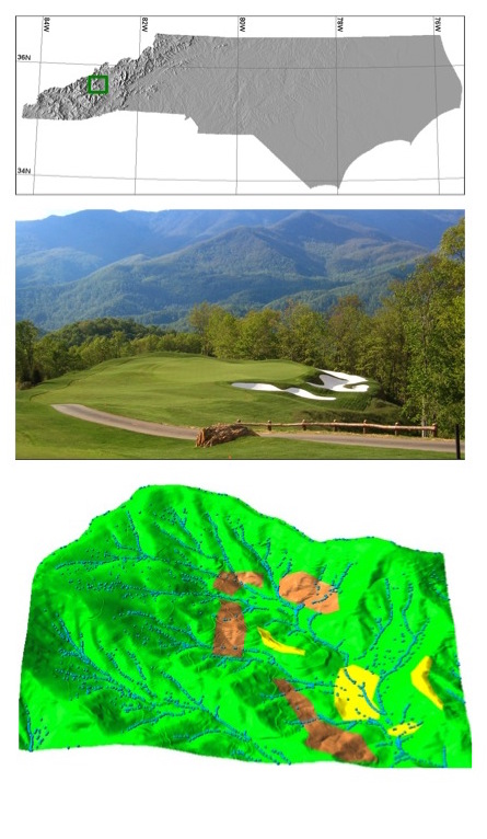
Surface flow modeling methods
- input: DEM with depression
- steady-state approximation: flow accumulation using least cost path
- D-inf flow accumulations with depression as sink
- kinematic wave: water accumulates is depression
- diffusive wave: water fills depression and flows out
- diffusive wave with predefined channel through depression
Water depth is represented as a surface in 3D to highlight the differences in methods
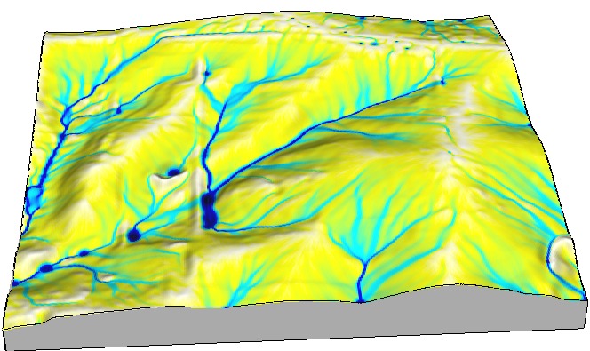
Dynamic surface flow modeling
Shallow water flow modeling with diffusion term using path sampling method:
Path sampling method
Solution of SWF equation is based on duality between particle and field representation: water depth is a function of particle density 
Particles show single impulse, water depth shows accumulated depth
Evolution of water depth
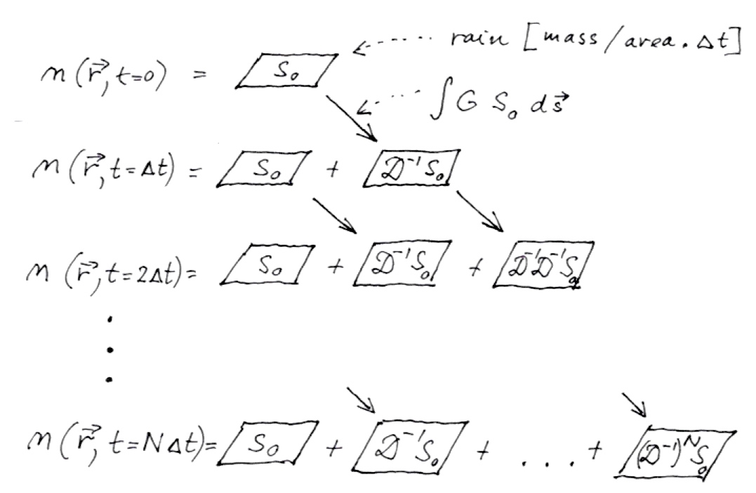
Path sampling method for SWF
Steady-state diffusive wave is approximated by a kinematic wave with approximate diffusive wave effects $ \propto \nabla^2 [h^{5/3}({\bf r})]$ :$$-{\varepsilon({\bf r})\over 2 }\nabla^2 [h^{5/3}({\bf r})] +\nabla \cdot [ h({\bf r}){\bf v}({\bf r})] = i_e({\bf r})$$
the solution is found by routing the particles, where the new position of m-th particle is computed as: $${\bf r}_m^{new} = {\bf r}_m + t{\bf v(r)} + {\bf g(r)}$$ where ${\bf r}_m = (x,y)$ is position of a particle, ${\bf v}$ is velocity vector, $t$ is time step and ${\bf g}$ is a random vector with Gaussian distribution around ${\bf r_m}$.
Evolution of water depth
Geometry-based (D-inf SFD) approximation: steady, uniform rainfall, constant velocity
Evolution of water depth
Path sampling solution during and after storm with diffusive flow on alluvial fan
Path sampling method
Solution of SWF equation incorporates spatially variable flow velocity- variable rainfall excess (impact of soils and land cover on infiltration),
- topography (slope steepness)
- land cover (Mannings roughness coefficient)
Applications for different types of landscapes
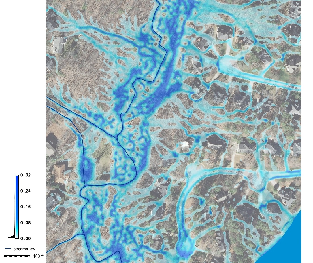
Urban flooding: sub-meter resolution
Path sampling solution for overland flow: with uniform rainfall and land cover, approx. diffusive wave
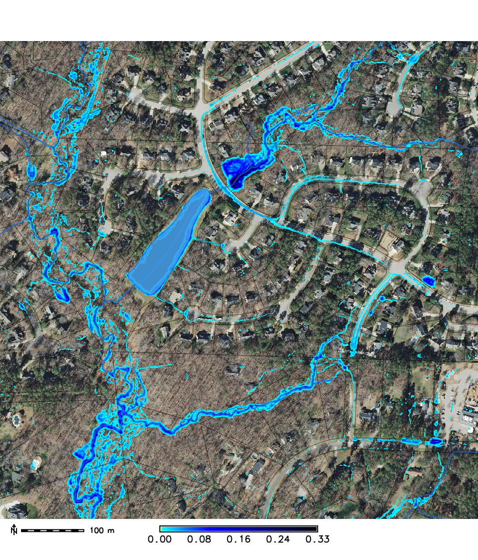
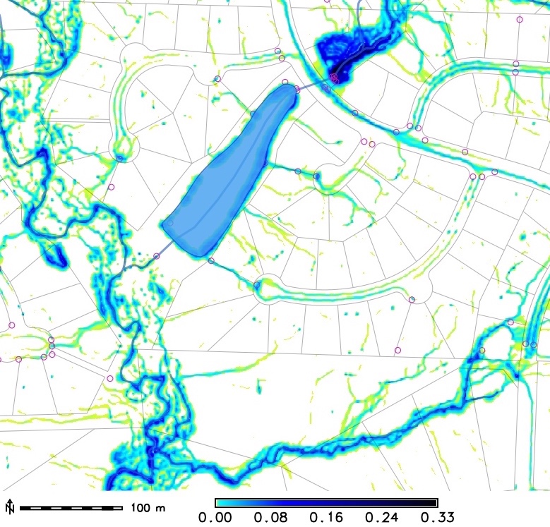
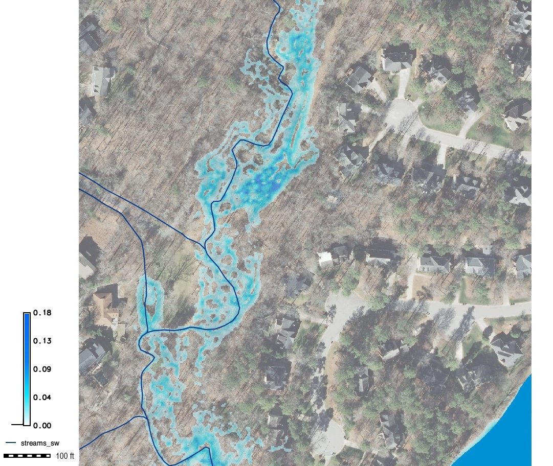
Urban flooding: sub-meter resolution
Extreme storm and post-storm water depth in a floodplain
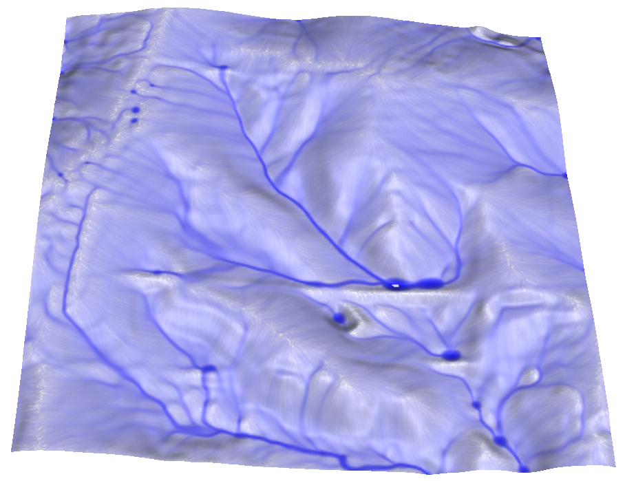
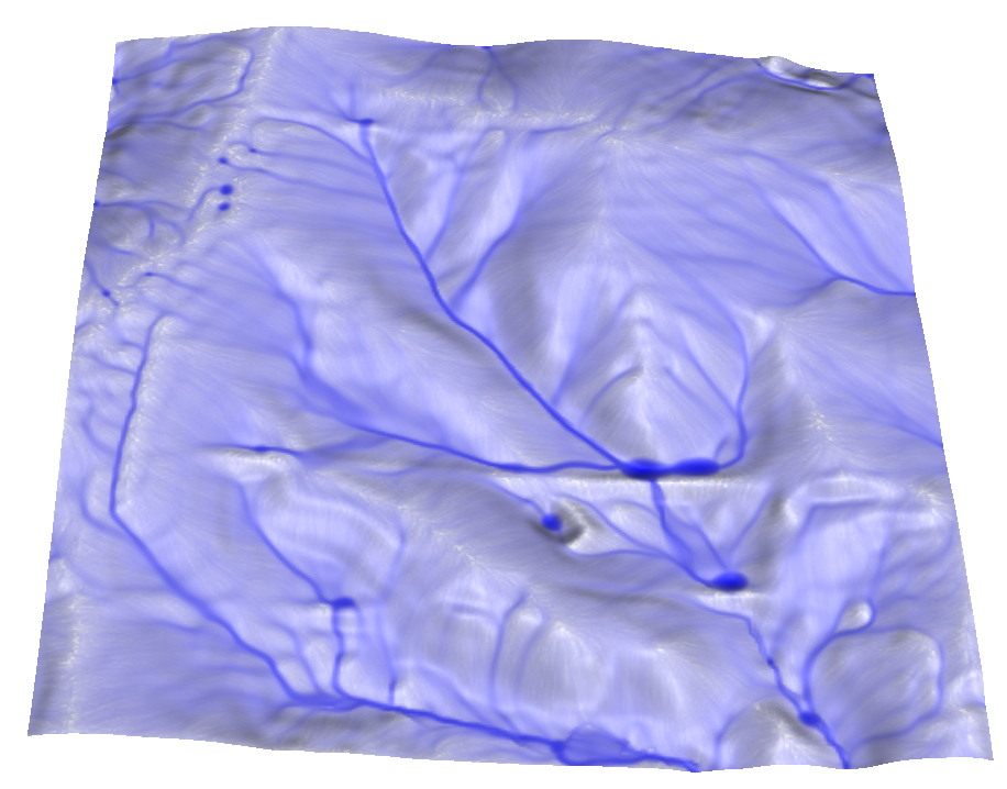
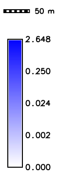
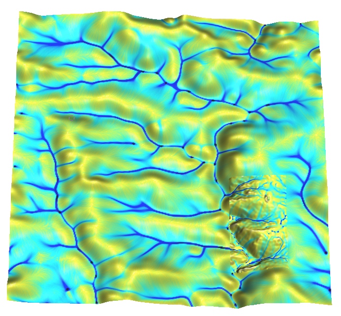
Landscape with pits
Surface water simulation in a landscape with numerous depressions
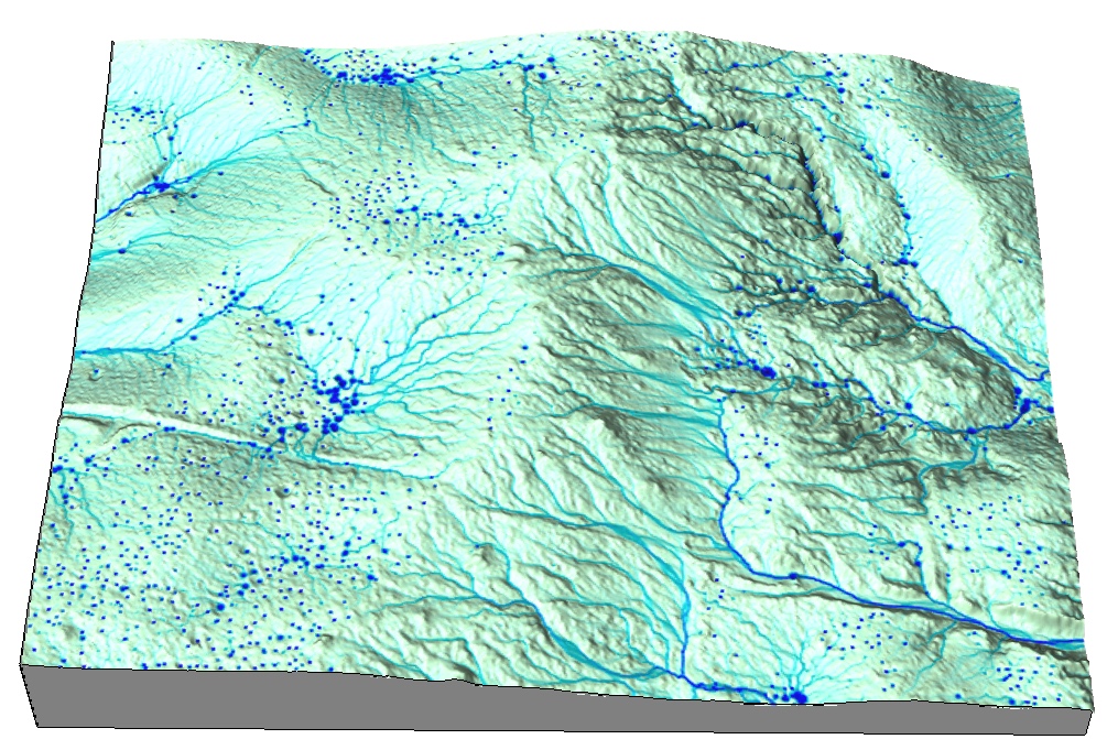
1m resolution DEM, most craters are diminished at 10m resolution
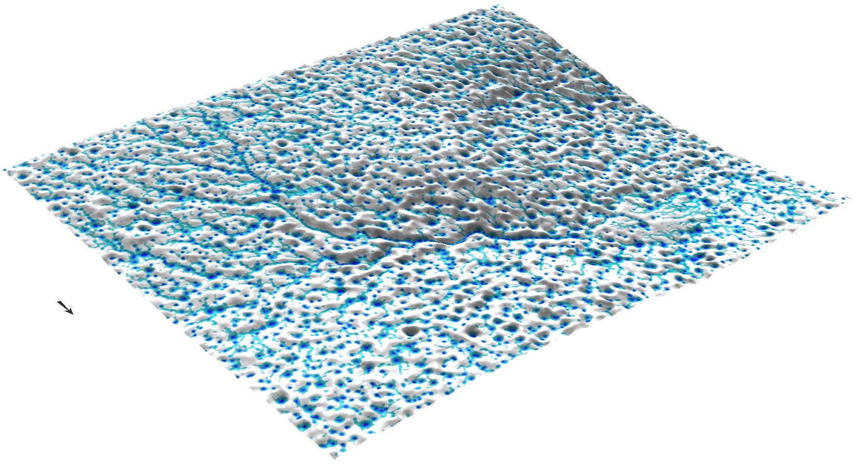
Overland flow with microtpography
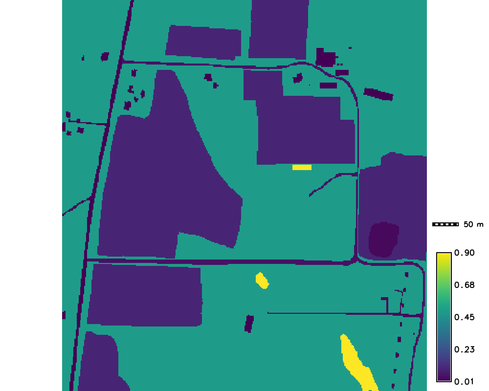
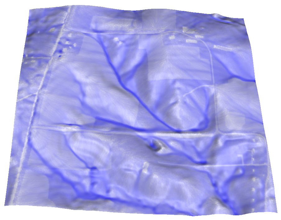
Surface water at ultra high resolutions (0.3m): tilled field
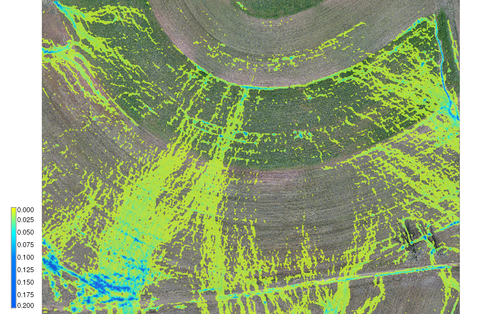
At lower resolutions, the tillage is represented by appropriate Mannings coefficient
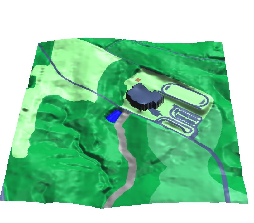
Development with storm water controls
Overland flow with spatialy variable land cover and storm water control measures: constructed wetland and checkdams
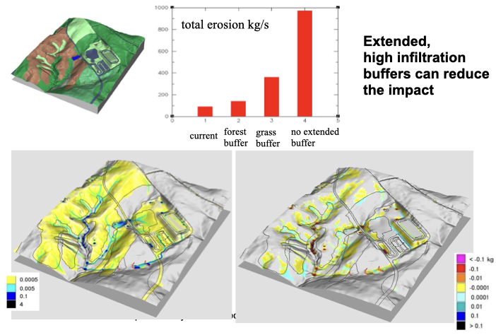
Impact of construction
Scenarios with spatialy variable land cover due to construction and land change where stream buffers offer only limited protection
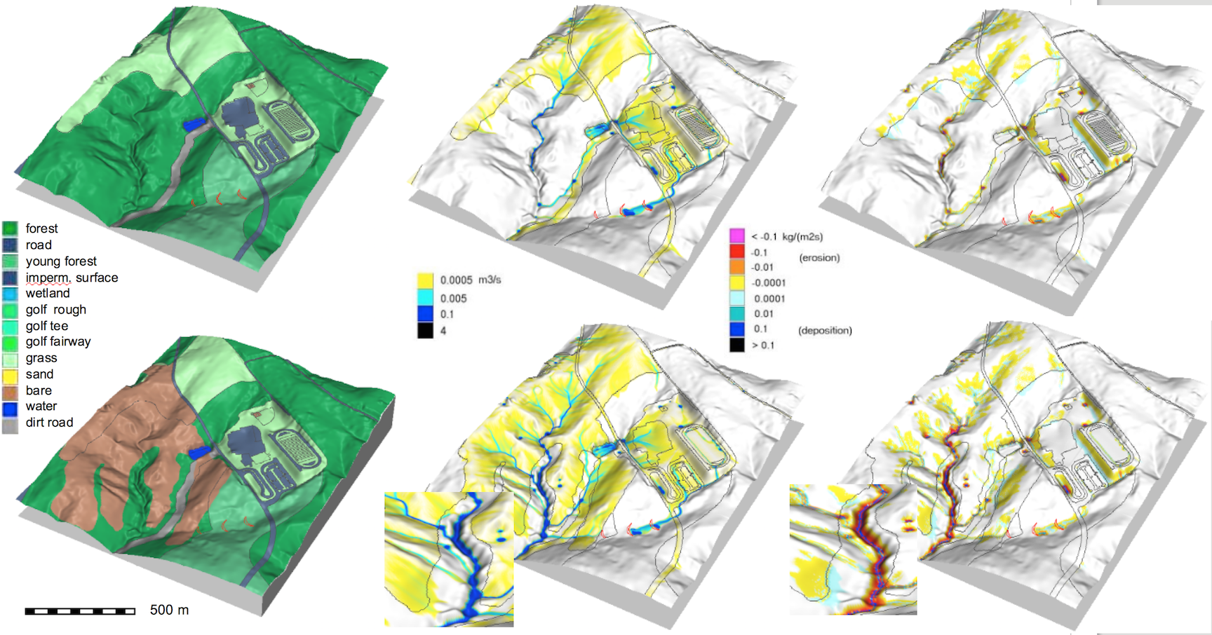
Impact of construction
Scenarios with spatialy variable land cover due to construction and land change where extension of stream buffers upstream improves protection
Dynamic wave applications
Dam breach model - full dynamic wave solution with backwater effect, using finite volume method
see supplemental material for equations and r.damflood manual page for references
Assignment
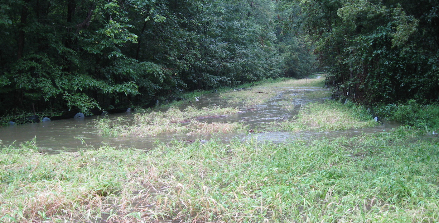
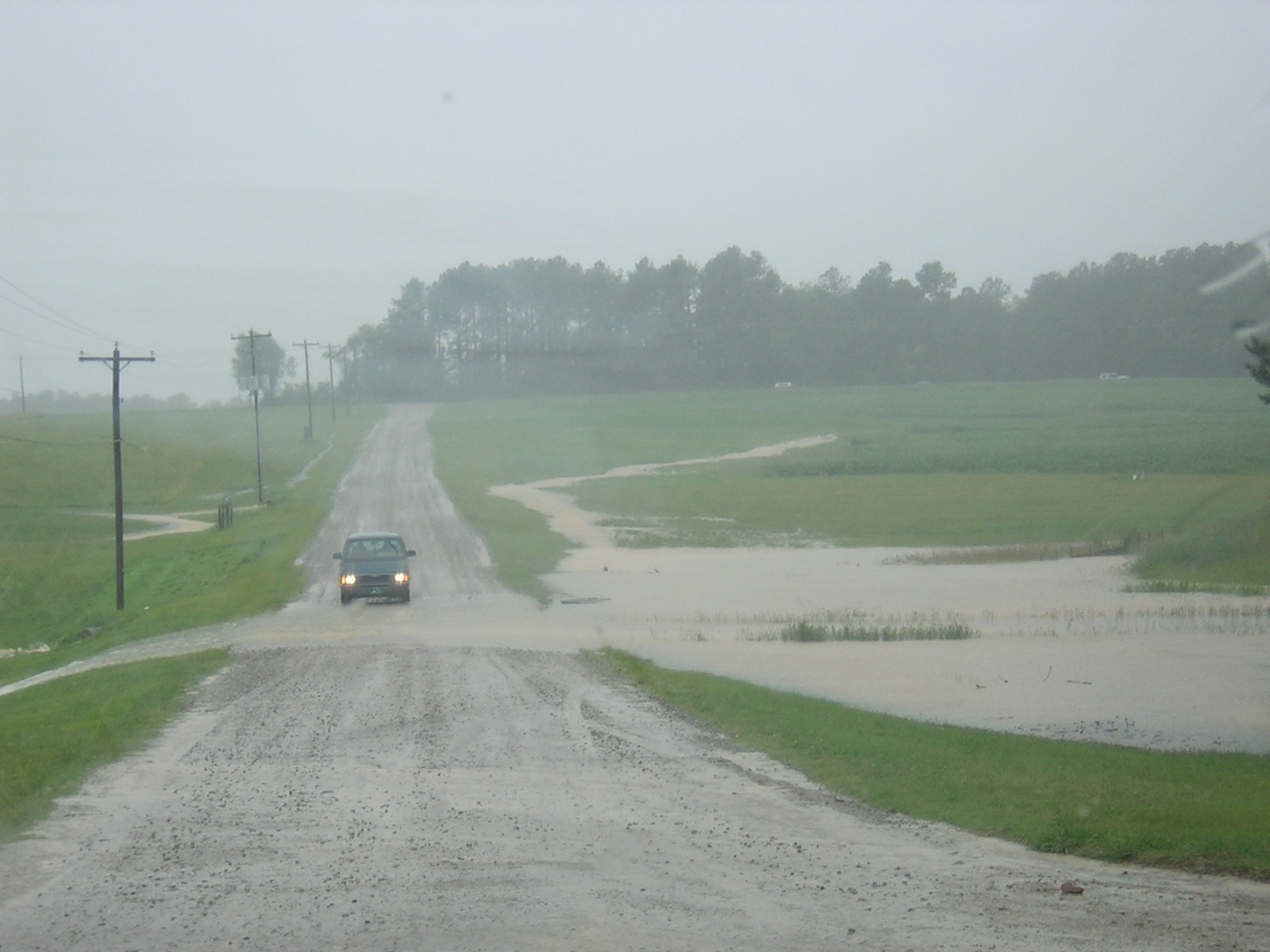
Surface water during hurricane Alberto
Assignment
Surface water during hurricane Alberto
Assignment
Surface water flow with uniform cover and enforced channel
Assignment
Coupling DEM-based gradient with enforced channel: ${\partial z \over \partial x}$ from DEM is replaced with ${\partial z \over \partial x}$ from the stream in grid cells where stream is located using map algebra
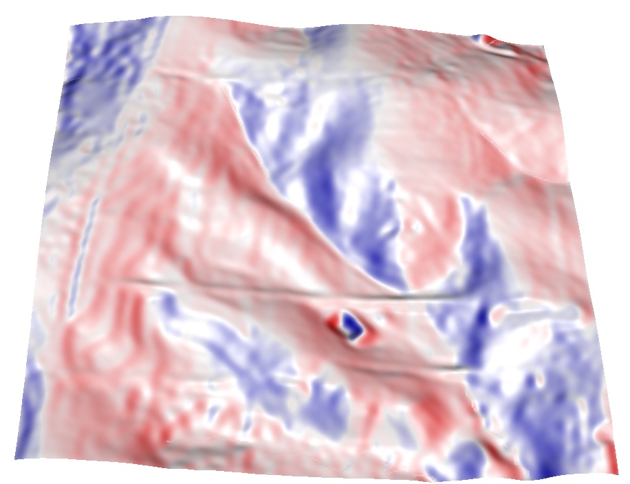
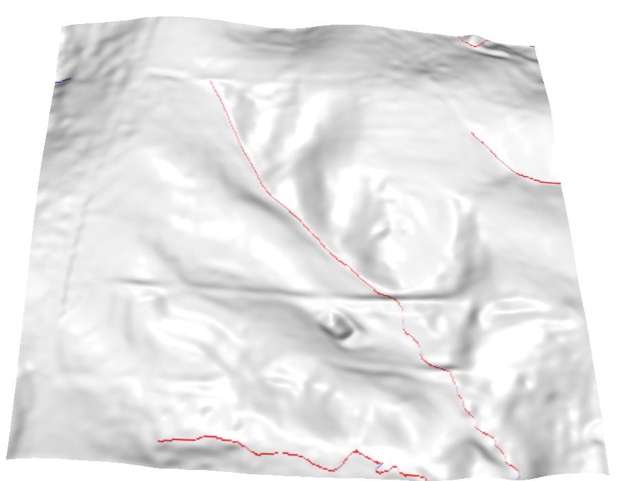
same is applied to $y$ direction
Assignment
Spatially variable land cover: increased roughness and reduced runoff
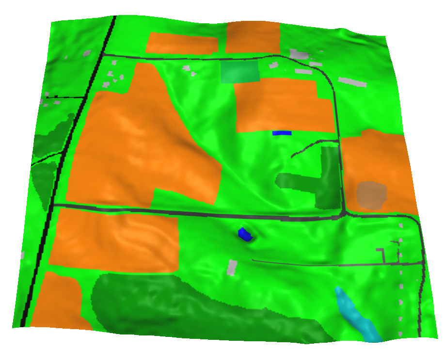
Assignment
Rainfall excess rate $<5,50>$, Mannings roughness $<0.01,0.5>$
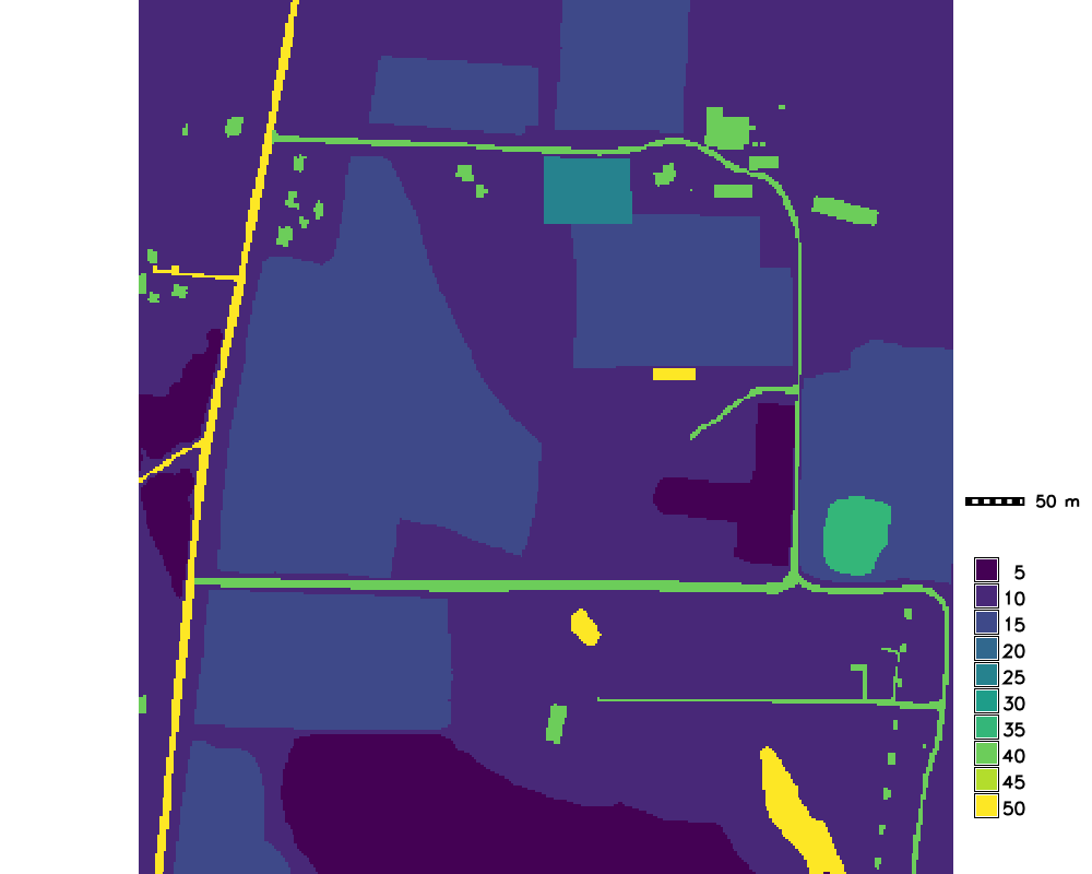
Assignment
Spatially variable land cover: increased roughness and reduced runoff
Few additional notes about path sampling method
Pluvial and fluvial flooding
Simulation of flodding from HAND method (inundation from a stream) and path sampling SIMWE method (overland flow)
Path sampling method: accuracy
Error is proportional to the $1/\sqrt N$, where N is the number of particles

Path sampling method: accuracy
Error is proportional to $1/\sqrt N$, $N$ is number of particles
Multiscale implementation
Path sampling enables implementation with multiple resolutions by adjusting the weight of the particles
Summary
- we defined surface water flow modeling components
- we introduced shallow water flow equations (SWFE)
- we explored applications of (SWFE)
- we visualized surface water flow dynamics