FUTURES
FUTure Urban-Regional Environment Simulation
Anna Petrasova, Vaclav Petras
GIS714 Geosimulations NCSU
FUTURES
(Meentemeyer et al., 2013)- urban growth model
- patch-based
- stochastic
- accounts for location, quantity, and pattern of change
- positive feedbacks (new development attracts more development)
- allows spatial non-stationarity
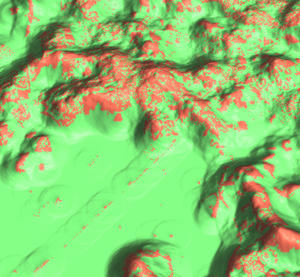
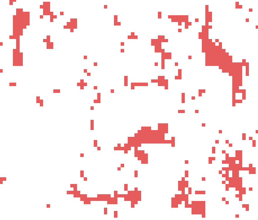
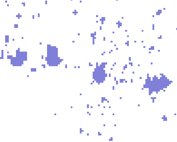
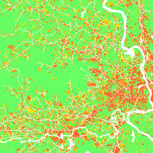
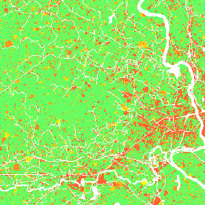
FUTURES, A Simplified View
turning green cells into orange cells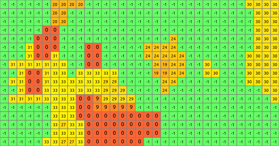
-1: undeveloped, 0: initial development, 1: developed in the first year, …
Modeling framework
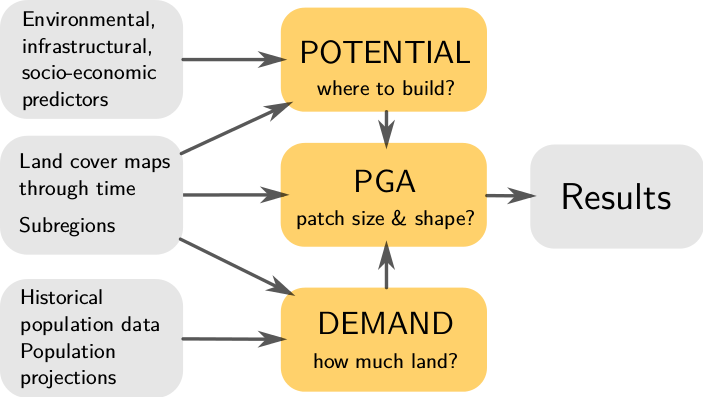
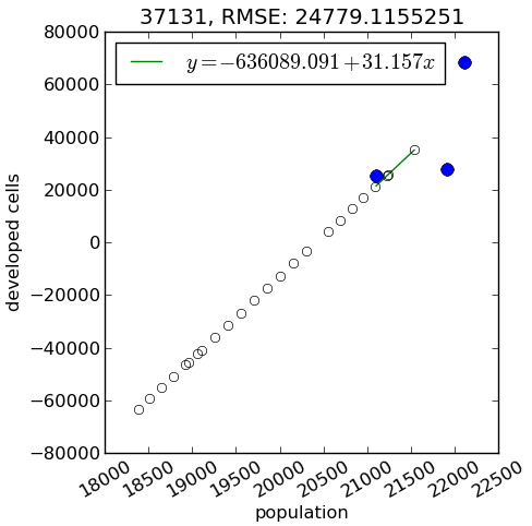
Demand submodel
- estimates the rate of per capita land consumption for each subregion
- extrapolates between historical changes in population and land conversion
- inputs are historical landuse, population data, population projection
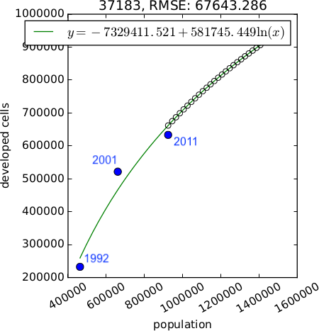
Demand scenarios
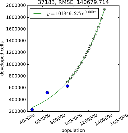
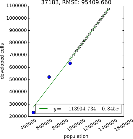
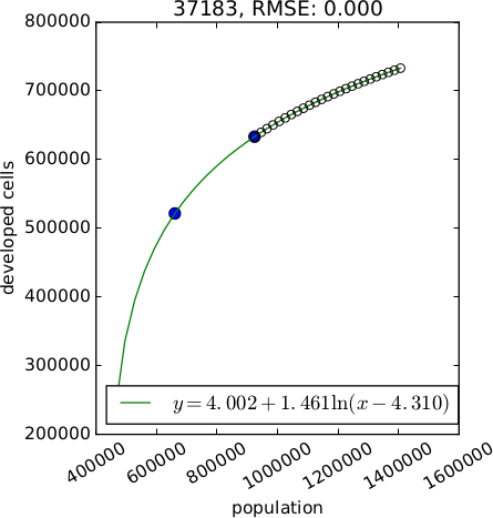
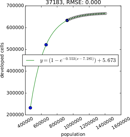
$$
y = Ae^{BX} \\
y = A + Bx \\
y = A + B ln(x) \\
y = A + B ln(x - C) \\
y = (1 - e^{-A(x - B)}) + C
$$
Demand: population decline
- demand submodel designed for regions with population growth
- FUTURES doesn't simulate cell de-conversion: here it would simulate zero new cell conversions
- even with population decline, impervious areas can increase
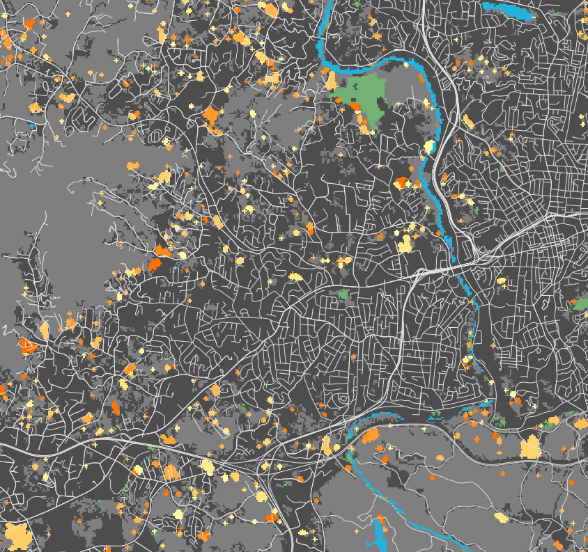
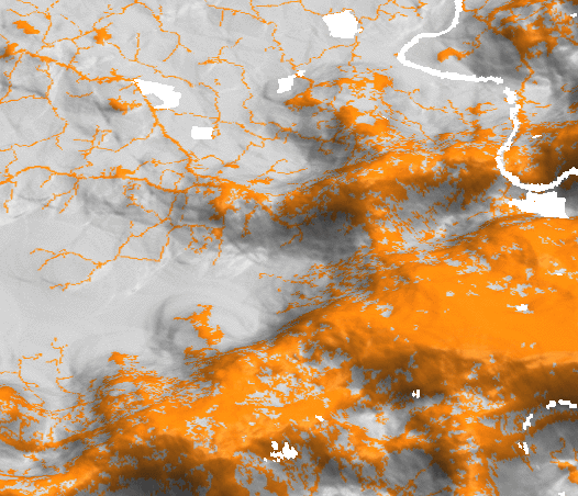
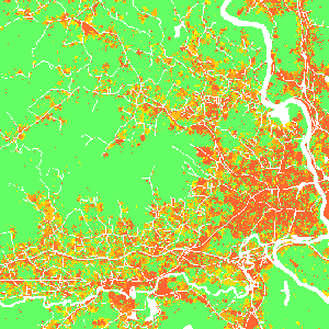
Potential submodel
- multilevel logistic regression for development suitability accounts for variation among subregions (for example policies in different counties)
- inputs are uncorrelated predictors (distance to roads and development, slope, ...)
surface: potential, orange: developed areas, green: undeveloped areas
Potential submodel
$$
p_i = \frac{e^{s_i}}{1 + e^{s_i}}
$$
$p_i$ is development probability for cell i,
$s_i$ is development potential for cell i
$s_i$ is development potential for cell i
$$
s_i = a_{j,i} + \sum_{h=1}^{n} \beta_{j, i, h} \, x_{i, h}
$$
$j$ is the level (e.g. counties),
$h$ is a predictor,
$n$ is the number of predictor variables,
$a_{j,i}$ is intercept,
$\beta_{j, i, h}$ is regression coefficient,
$x_{ih}$ is the value of h at i
$h$ is a predictor,
$n$ is the number of predictor variables,
$a_{j,i}$ is intercept,
$\beta_{j, i, h}$ is regression coefficient,
$x_{ih}$ is the value of h at i
Potential submodel: workflow
- stratified random sampling of predictors and response variable (developed/undeveloped raster)
glm(developed ~ (1|subregion) + distance_to_water + development_pressure + road_density + ...)- using automatic selection based on AIC
- create probability surface from regression coefficients
Potential submodel: notes
- predictors and coefficients do not change during simulation (except for development pressure)
- avoid multicollinearity
Development pressure
- Predictor based on number of neighboring developed cells within search distance, weighted by distance.
- Allows for a feedback between predicted change and change in subsequent steps.
where $state_k$ indicates whether $k$th neighboring cell is 1 or 0 (developed or undeveloped)
$d_{ik}$ is distance between current cell $i$ and neighboring cell $k$
and $\gamma$ controls the influence of distance between neighboring cells
Development pressure
Patch Growing Algorithm
- stochastic algorithm
- converts land in discrete patches
- inputs are patch characteristics (distribution of patch sizes and compactness) derived from historical data
Patch Growing Algorithm
- pick randomly a seed cell $i$
- seed is established if $p_i$ > random number
- randomly pick patch size
- grow patch
- add neighbors to a list and sort it based on $p_i / d^c$, where $d$ is distance from $i$ and $c$ is compactness value
- pick first neighboring cell and try to add it to the patch if $p_i$ > random number
- if added, add surrounding neighboring cells to the list
- repeat until the patch size is met
- recompute development pressure
Patch Compactness
Low
High
Scenarios: Incentive power
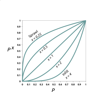
Scenarios
Constraint parameter: zones with decreased probability of development $$P_{new} = P . C, \quad C \in \langle 0, 1\rangle $$Stimulus parameter: zones with increased probability of development $$P_{new} = P + S - P.S, \quad S \in \langle 0, 1 \rangle$$
r.futures
Information flow diagram for the set of modules implementing FUTURES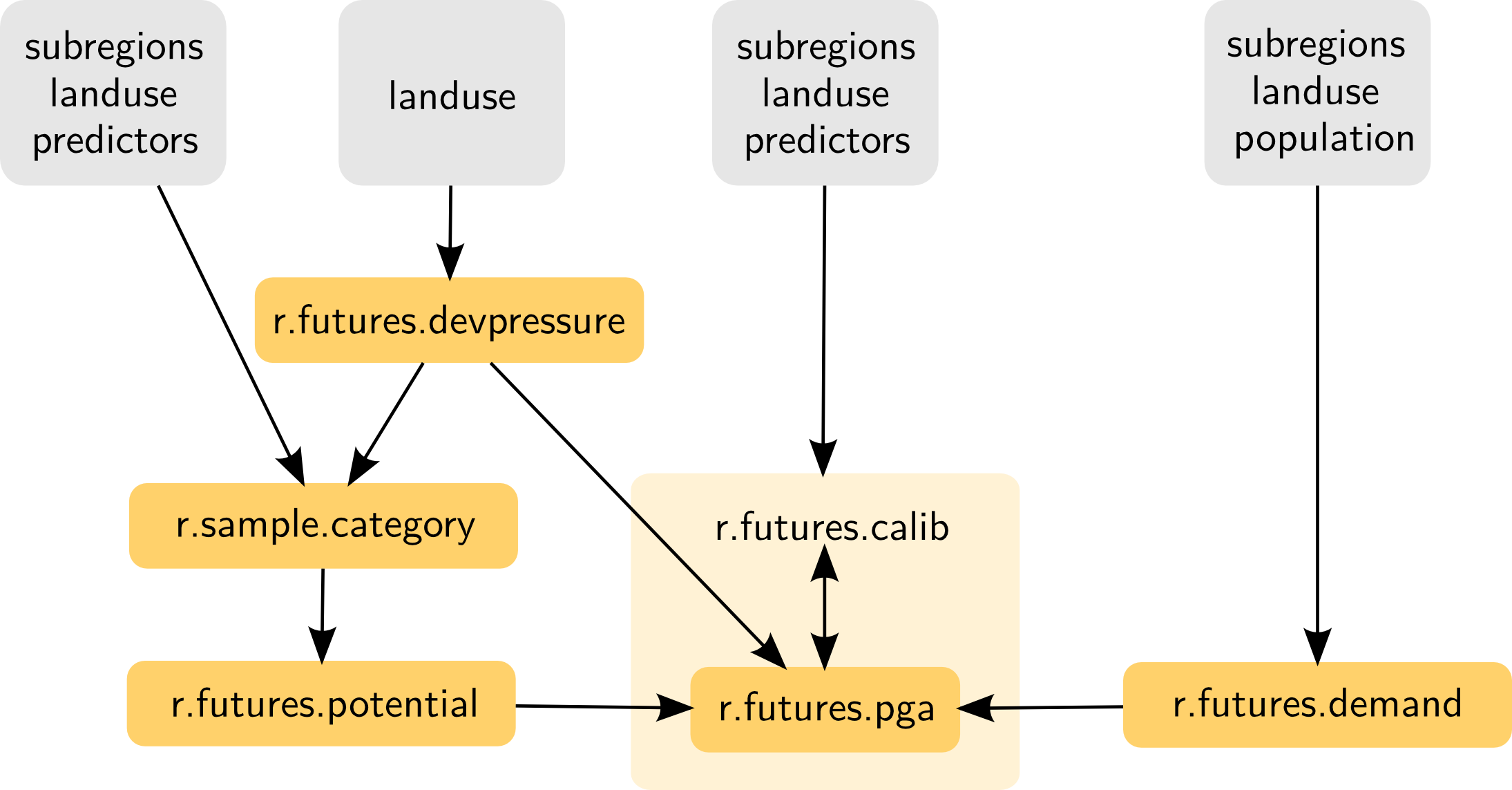
Additionally, r.futures.parallelpga can be used instead of r.futures.pga.