Pest or Pathogen Spread Modeling

Anna Petrasova, Vaclav Petras, Devon Gaydos, Chris Jones,
Helena Mitasova

GIS714 Geosimulations NCSU

Motivation

• Plant diseases and pests threaten production of food and plant-based materials
• NCSU CGA & USDA APHIS developing tools to forecast the spread of pests and pathogens and to design effective control measures

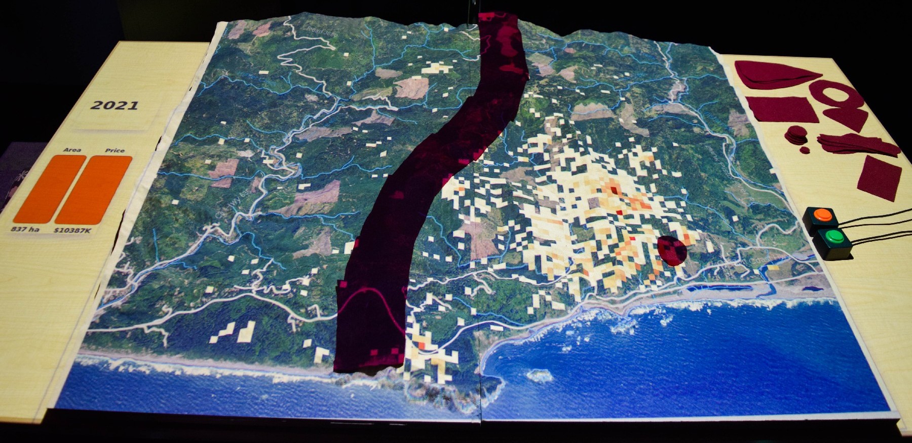
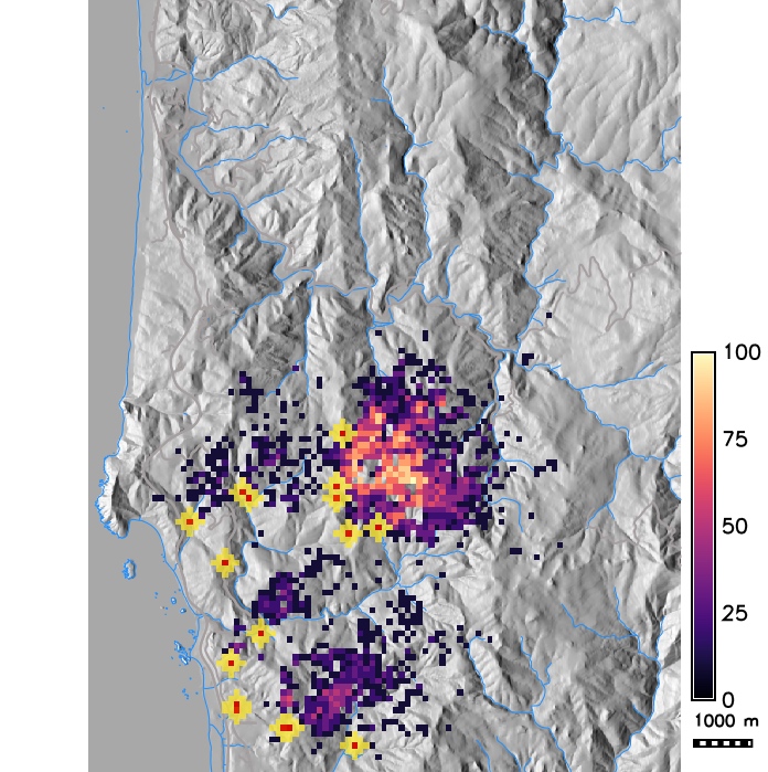
Spotted lantern fly infestation

Modeling components

• Modeled quantity [units]: density of infected plants (hosts)
• Spatial and temporal extent and scale: field, regional, global spread
• Configuration space and interactions: host density, weather, initial infected locations
• Governing equations or rules: rate of reproduction, distance and direction of spread, establishment

Pest or Pathogen Spread Model PoPS

Geospatial simulation of pests or pathogens over a landscape

Main drivers:

• locations with infected hosts
• host density
• weather conditions

Main outputs:

• Spatial distribution of infected host densities at a given time
• Spatial distribution of infected host probabilities over time

PoPS model description

Governing equation

$$ \Psi_{ijt} = \beta W_{it} I_{it} * K (d, w) * (W_{jt} S_{jt}) / N_j$$

where

• $\Psi_{ijt}$ is number of infested hosts in cell $j$ as a result of pest dispersal from cell $i$
• $\beta$ number of pests/pathogens from a single host under optimal conditions
• $W_{it}$ is weather in cell $i$, $I_{it}$ number of infected hosts in cell $i$
• $K (d, w)$ is the dispersal as a function of distance parameters $d$ and wind properties $w$
• $W_{jt}$ is weather in cell $j$, $S_{jt}$ number of susceptible hosts in cell $j$,
• $N_j$ number of all potential hosts in cell $j$

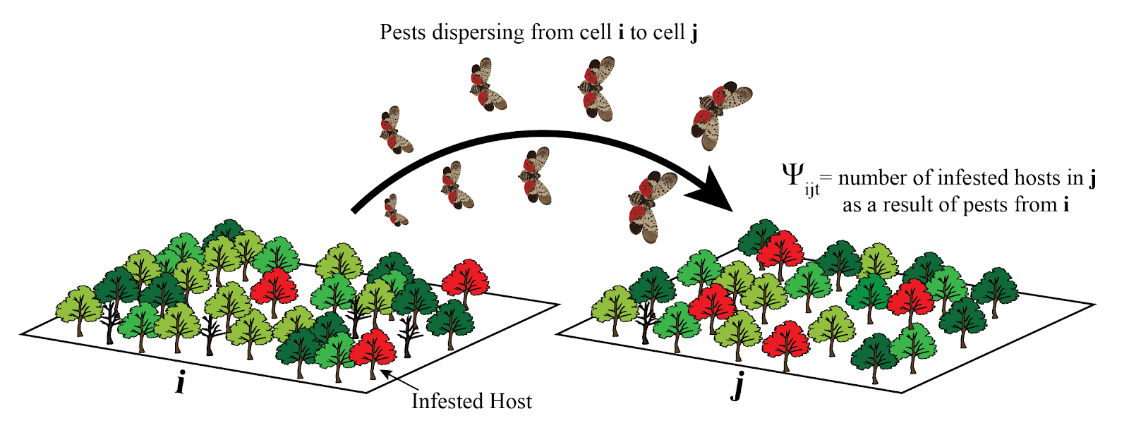
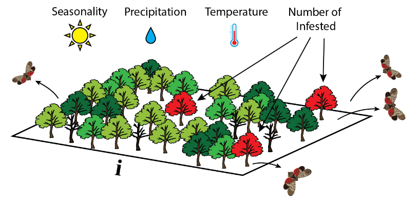
Generating pests/pathogens: reproduction

$$\lambda = \beta X_{it} P_{it} T_{it}$$

where

• $\beta$ number of pests/pathogens from a single host under optimal conditions
• $X_{it} P_{it} T_{it}$ is weather: seasonality, precipitation, temperature
• weather is implemented as weather coefficient derived from historical weather data
• number of pests/pathogens is randomly selected from Poisson distribution

Spreading the pests/pathogens: dispersal

$$ V_{ij} = K(d_{ij}; \alpha_1, \alpha_2, \gamma, D(\omega, \kappa))$$

where

• $d_{ij}$ is distance
• $\alpha_1, \alpha_2$ are short and long distance dispersal scales
• $\gamma$ is percent short distance dispersal
• $D$ is the wind vector with direction $\omega$ and strength (magnitude) $\kappa$
• distance is selected from Cauchy distribution, wind direction is from von Mises (circular normal) distribution

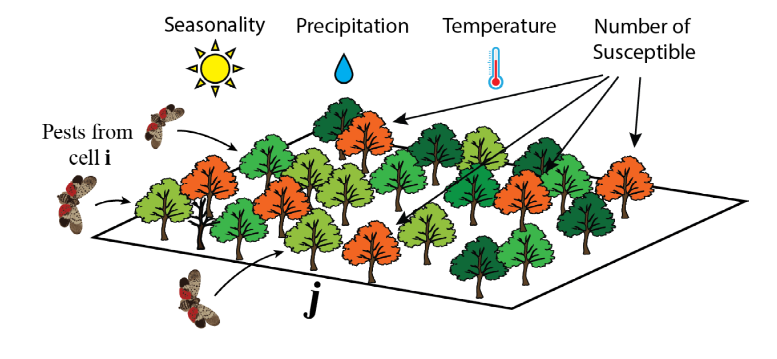
Establishment of pests/pathogens

$$E_j = X_{jt} P_{jt} T_{jt} S_{jt}/N_j $$

where

• $S_{jt}$ is the number of susceptible hosts in cell $j$ and $N_j$ is the number of all hosts in cell $j$
• $X_{jt} P_{jt} T_{jt}$ is weather: seasonality, precipitation, temperature in cell $j$

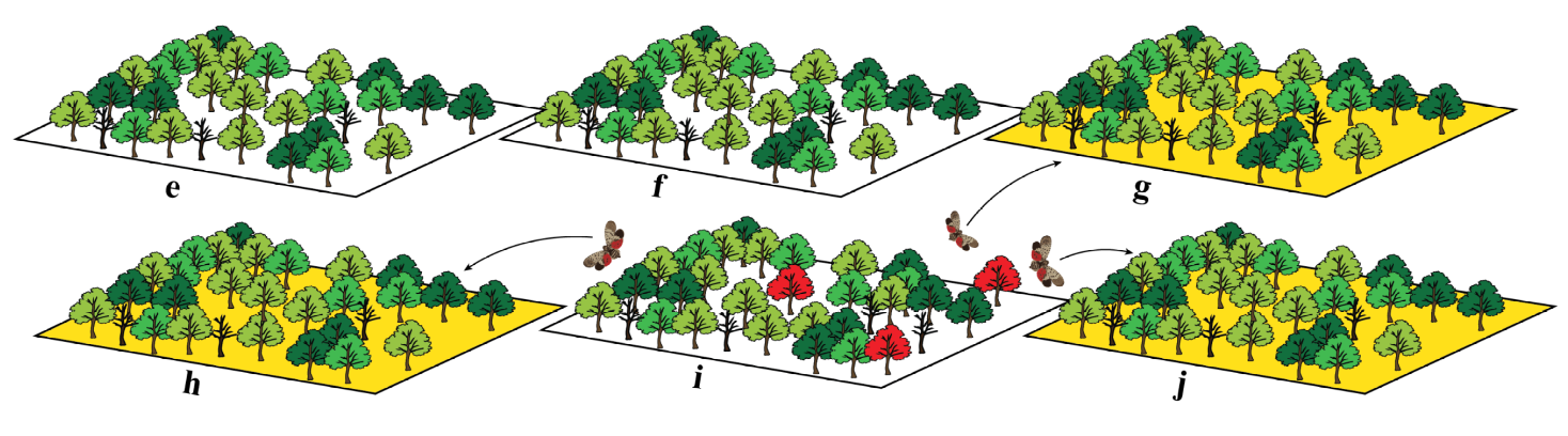
Spatial outputs of stochastic simulations

• Number of infected hosts (trees, plants) in each cell from individual stochastic runs
• Probability infection map: probability that the hosts will be infected over given period of time derived from large number of stochastic runs
• Average number of infected hosts in each grid cell from large number of stochastic runs and associated standard deviations map

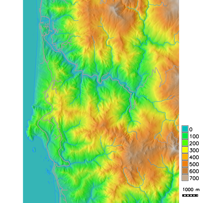
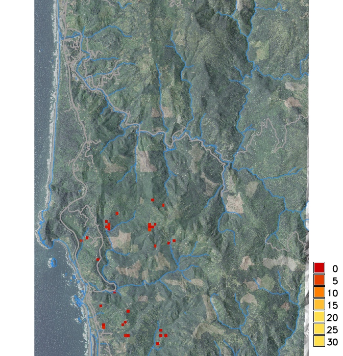
PoPS application for SOD modeling

Study area and initial locations with hosts infected by a pathogen causing Sudden Oak Death (SOD) disease

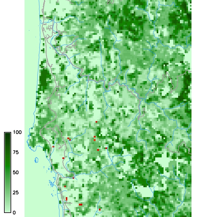
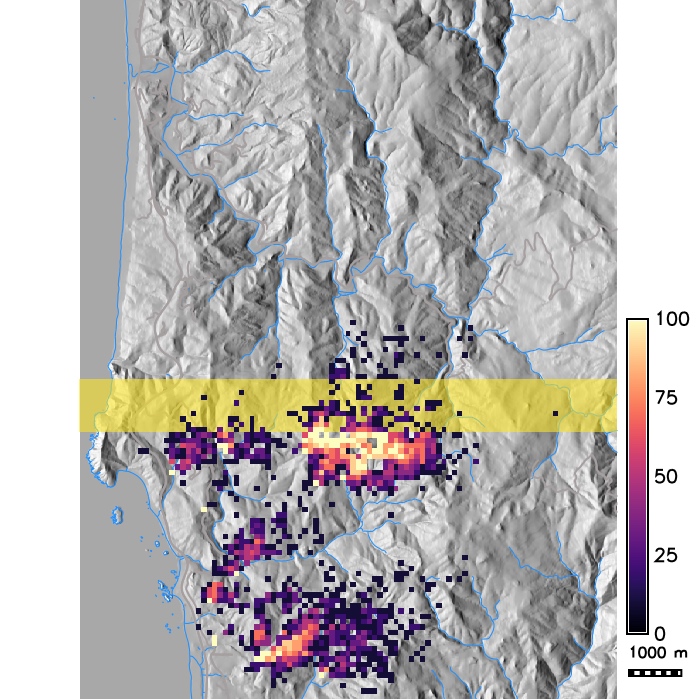
PoPS application for SOD modeling

Host density and a weather index map

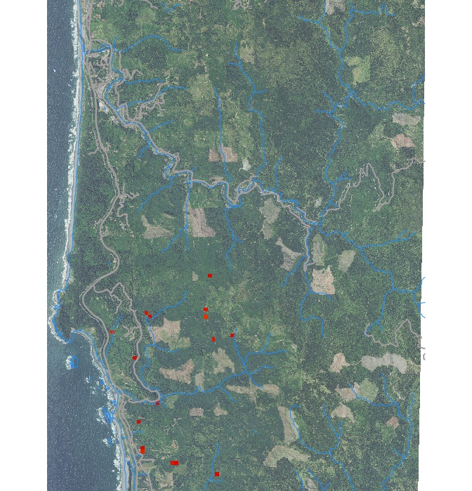
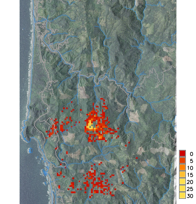
PoPS application for SOD modeling

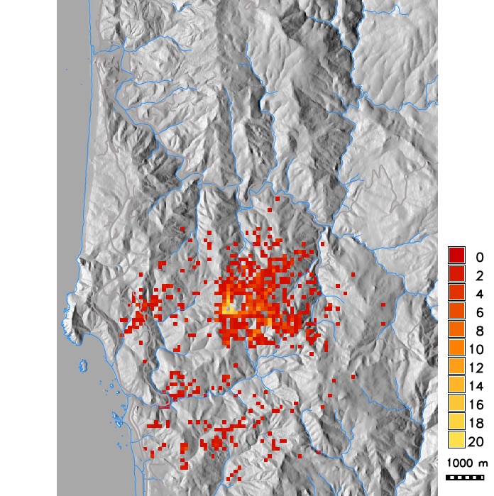
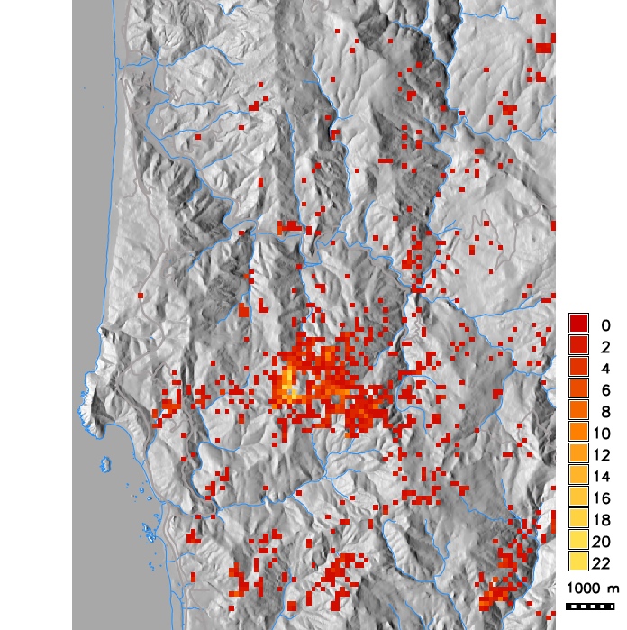
Infected hosts in 2019 and 2023 from a single stochastic run

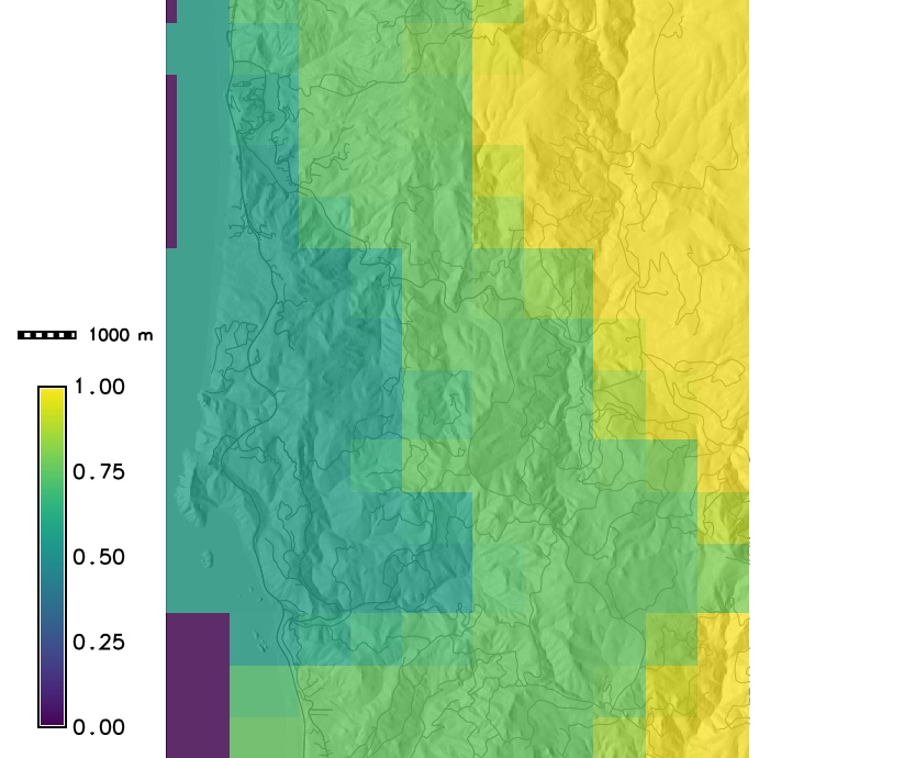
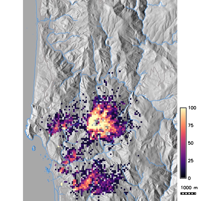
PoPS application for SOD modeling

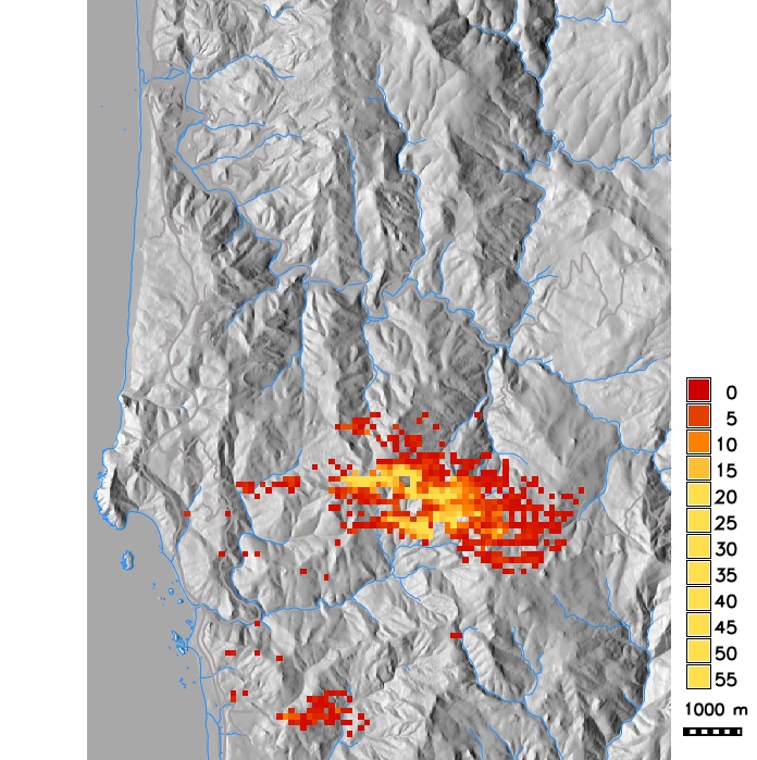
Probability of grid cell getting infected as a result of many stochastic runs and average number of infected trees per grid cell

Scenario modeling

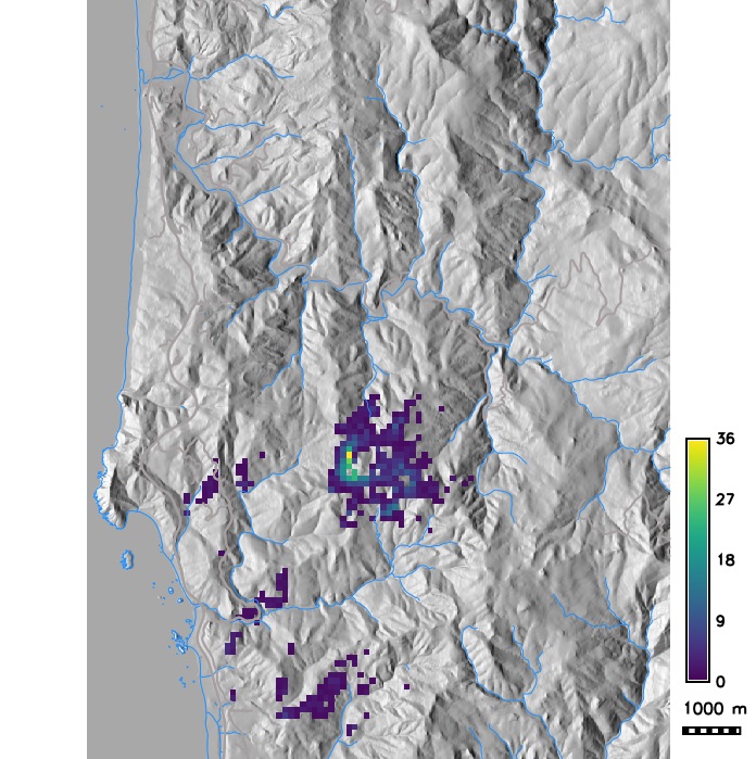
PoPS application for SOD scenario modeling

Number of infected hosts per cell from single run simulations with different dispersal kernels (exponential with modified distance and wind strength, Cauchy, anisotropic)

PoPS application for SOD scenario modeling

Probability of hosts getting infected in a grid cell for management scenarios: local buffers, massive barrier clear cut

Software

• PoPS (C++ library)
• rpops R package (uses Rcpp for R C++ integration)
• r.pops.spread GRASS GIS Addon in C++

All open source, hosted on GitHub

User Interfaces

• PoPS Web Platform
• Tangible Landscape

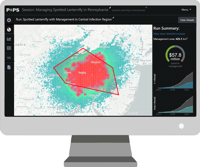
PoPS Forecasting and Control System

Interconnected components:

• PoPS model: predicts probability of infection
• Spatial Decision Support System: interactive dashboard for stakeholders
• Iterative sampling and management: validation of forecasts and improving calibration
• Pest/Pathogen parameter library: biological characteristics influencing spread
• Host map library: satellite data + machine learning algorithms

Calibration and validation

What are the correct parameters for this model?

Calibration is the estimation and adjustment of model parameters and constraints to improve the agreement between model output and a data set

How does the model perform compared to the real system?

Validation is a demonstration that a model possesses a satisfactory range of accuracy consistent with intended application of the model

Calibration methods

• Monte Carlo Markov Chains (MCMC)
• Approximate Bayesian Computation (ABC)

Assumptions:

• Simulation and data are comparable (i.e., the output from the simulation is a quantity recorded in the data) or can be compared from summary statistics.

Calibration using MCMC

Markov Chains:

sequences of events that are probabilistically related to each other. Each event comes from a set of outcomes, and each outcome determines which outcome occurs next, according to some fixed probability set.

• They are memoryless: everything you need to know for the next state is available in the current state.
• Over the long run, it settles into a pattern.

Monte Carlo simulations

repeatedly generating random numbers to estimate some fixed parameter value

Calibration using MCMC

1. generate a random parameter set and run the model
2. if the new parameter performs better, it is added to the chain of parameter values with a certain probability determined by how much better it is
3. repeat this sequence many times to get a distribution of possible parameters
4. take the most common parameter from this distribution

Calibration using ABC

Generations

number of times to iterate

Particles

number of parameter sets to keep in each generation

Epsilon

the threshold that determines if a parameter set is kept or rejected

Calibration using ABC

1. Choose number of Particles (P)
2. Choose epsilon $\epsilon$
3. Calculate summary statistics for observed data $S_d$
4. Draw parameters from a uniform distribution
5. Run model
6. Calculate summary statistics for simulated data $S_s$
7. $D(S_d, S_s) ≦ \epsilon$
1. Keep (increase p by 1)
2. Else reject
8. Repeat 4 - 7 until p = P

Basic ABC example

Simple, but requires lot of user input to test for best $\epsilon$, computationally slow if $\epsilon$ is low.

Calibration using ABC-SMC

• a sequence of distributions is constructed by gradually decreasing $\epsilon$ in each generation ($\epsilon_1, \epsilon_2, \epsilon_3,$... can be pre-selected or derived based on the previous generation)
• each generation is obtained as a weighted sample from the previous distribution that has been perturbed through a kernel
• perturbation kernel can be uniform distribution, multivariate normal distribution

Calibration using ABC-SMC MNN

• ABC-SMC MNN uses multivariate normal distribution based on covariance matrix
• covariance matrix calculated using M nearest neighbors (MNN) of a particle
• normalised Euclidean distance can be used when searching for the nearest neighbours

Bayesian Updating

Quickly incorporate new data:

1. use previous posterior means and covariance matrix as priors for next time
2. use ABC_SMC MNN to calibrate for new year of data
3. calculate weights, e.g., based on number of observations
4. calculate posteriors from priors, calibrated parameters and weights

Comparison metrics

• Proportion of correct pixels
• Odds ratio
• Kappa
• Quantity disagreement
• Allocation disagreement
• Configuration disagreement

See Pickard et al. (2019)

Quantity and Allocation disagreement

Quantity disagreement = $|3 - 4| = 1$
Allocation disagreement = 2 (always even, here 1 pixel swapped)

Confusion matrix

Odds Ratio

$$\mbox{Odds ratio} = \frac{TP * TN}{FP * FN}$$

Issues with Odds Ratio

Kappa

$$\kappa = \frac{P_o - P_e}{1 - P_e}$$ $$P_o = \mbox{observed agreement} = \frac{TP + TN}{\mbox{All}}$$
$$P_e = \mbox{probability of random agreement} = P_{yes} + P_{no}$$
$$P_{yes} = \frac{TP + FN}{\mbox{All}} * \frac{TP + FP}{\mbox{All}}$$
$$P_{no} = \frac{FP + TN}{\mbox{All}} * \frac{FN + TN}{\mbox{All}}$$

Issues with Kappa

• Penalizes a map more strongly for allocation disagreement than quantity disagreement
• It’s a ratio, which can introduce problems in calculation and interpretation (e.g., when denominator or numerator is 0; is a value low because the denominator is high, or because the numerator is low?
• It compares to a random baseline, but this can be irrelevant or misleading. It might be more useful to compare to a naïve classification (like assuming no disease spread)

Landscape pattern

Simulations A and B have the same quantity and allocation disagreements, but A is more reflective of the truth.

Configuration disagreement

Combination of different metrics:

• Edge contrast
• Patch shape complexity
• Aggregation
• Nearest neighbor distance
• Patch dispersion
• Large patch dominance
• Neighborhood similarity

See Pickard et al. (2019), Cushman et al. (2008)

More about PoPS

• Sudden Oak Death spread modeling with PoPS
• PoPS website with on-line application
• GIS714 course material