Tangible Landscape as a geosimulation environment
Helena Mitasova, Anna Petrasova, Vaclav Petras
GIS714 Geosimulations NCSU
Learning objectives
- motivation for tangible simulation
- evolution of tangible simulation environments
- Tangible Landscape principle and setup
- creating 3D physical models
- tangible interactions
- Tangible Landscape applications
Motivation
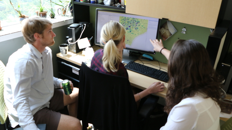
- Paper maps provide limited data with limited interaction, but encourage face-to-face discussion
- Digital maps limit f2f collaboration - only one user at a time can navigate and modify models.
- Interaction through mouse, keyboard and display does not encourage creativity.

Motivation
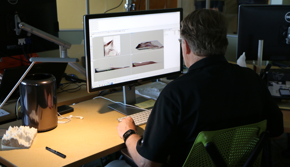
- Manipulating 3D computer models is not intuitive and requires specialized software and training.
- 3D physical models provide intuitive representation of landscapes but interaction is limited
Evolution of tangible interfaces
MIT Media Lab: URP (1999), Illuminating Clay (2004)


3D scanning with $40,000 laser scanner. Image source:
MIT Media Lab
Ishii H., Ratti C., Piper B., Wang Y., Biderman A. and Ben-Joseph E.
"Bringing clay and sand into digital design—continuous tangible user interfaces." BT technology journal 22.4 (2004): 287-299.
Underkoffler, J. Ishii, H. "Urp: a luminous-tangible workbench for urban planning and design", 1999,
CHI '99 Proc. SIGCHI conference on Human Factors in Computing Systems, p. 386-393.
TUI evolution: TanGeoMS
Tangible Geospatial Modeling System at NCSU (2007)

TUI evolution: AR sandbox
Augmented Reality Sandbox with $100 Kinect
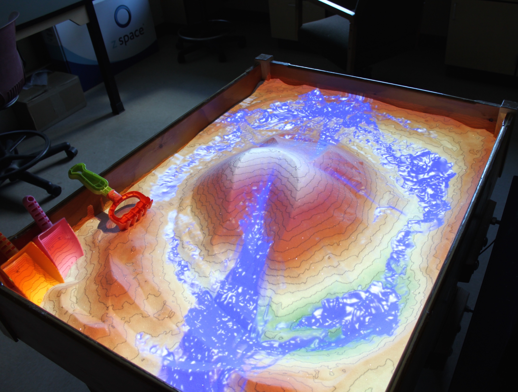
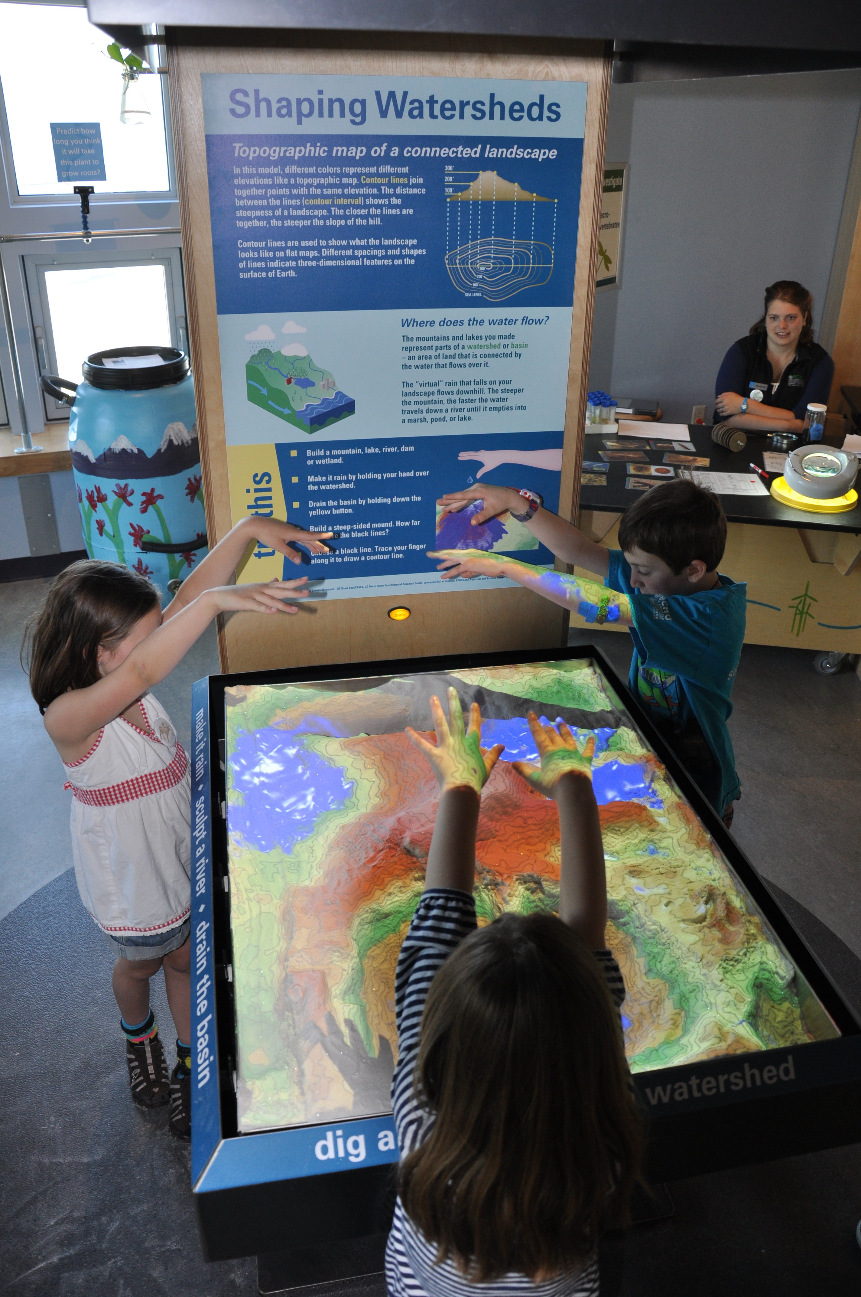
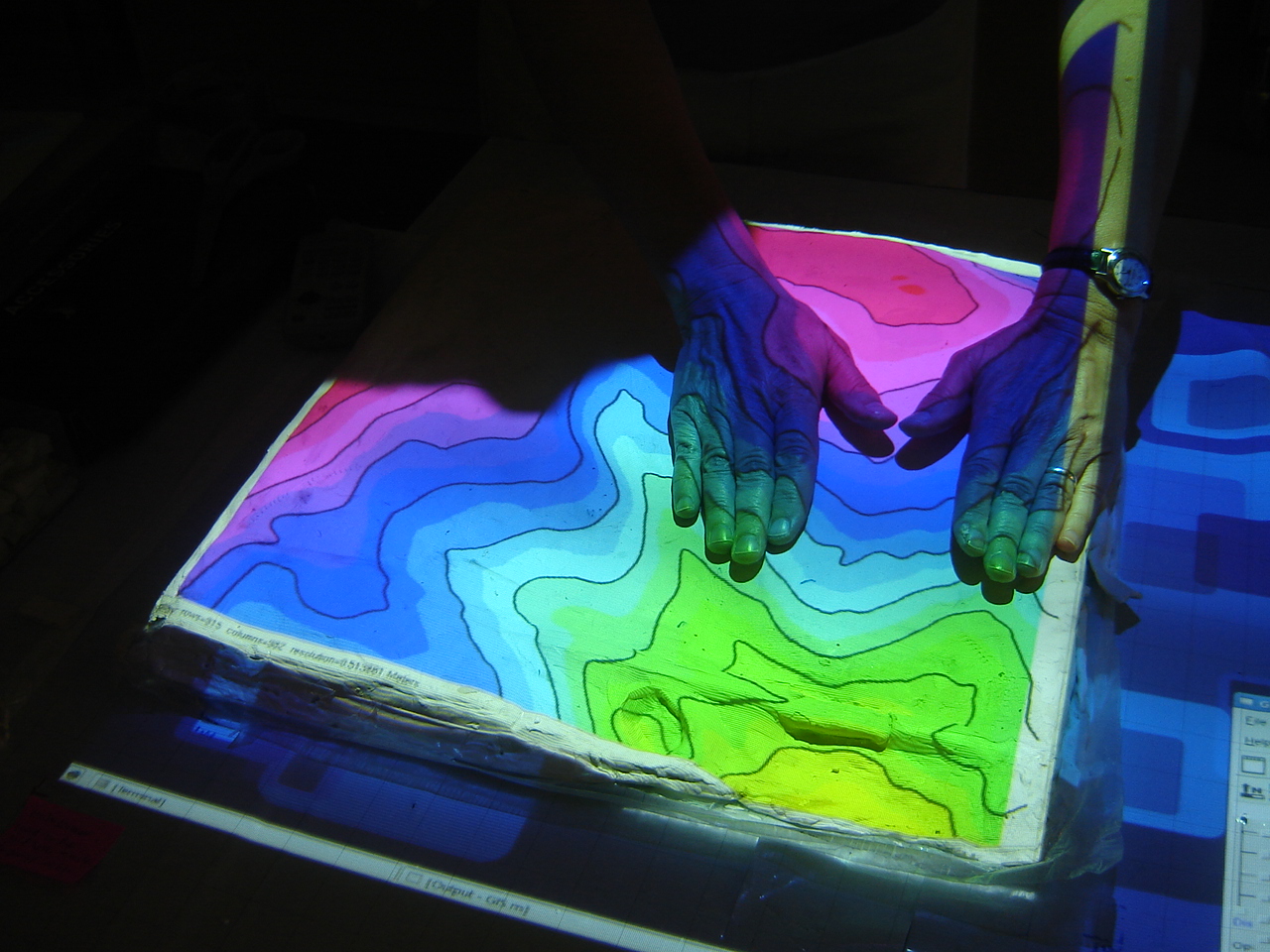
Tangible Landscape
Real-time coupling with GIS: simulation system
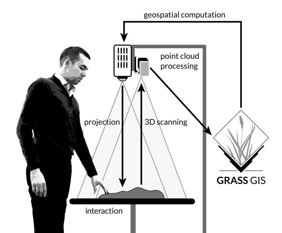
Tangible Landscape couples a digital and a physical model through continuous cycle of 3D scanning, geospatial modeling, and projection.
Software architecture

Software architecture
Extended system with 3D rendering and virtual reality
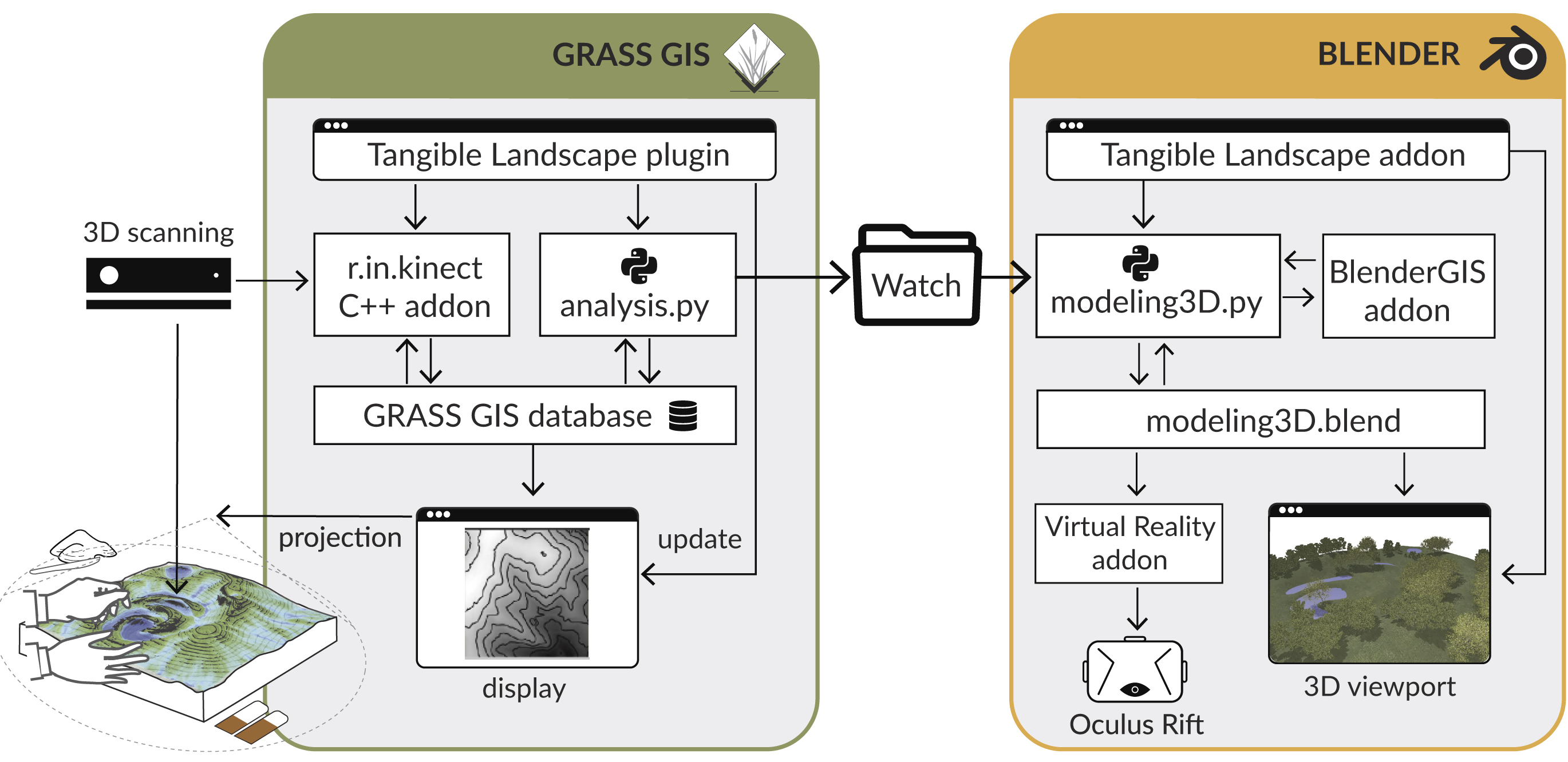
Software architecture
System roles: user, operator, developer
Physical 3D models
What are your suggestions for creating 3D models?
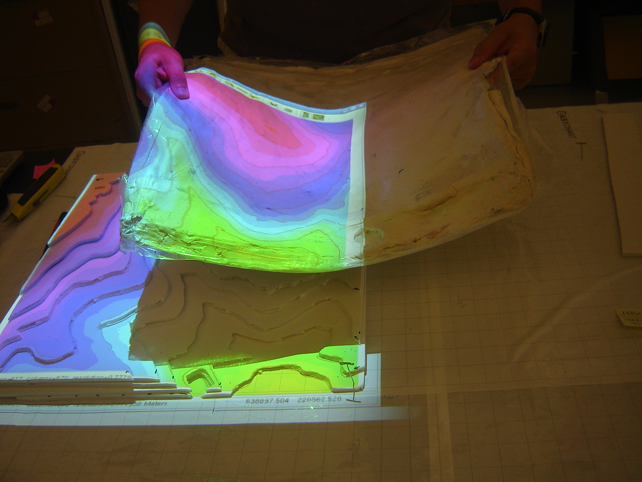
Contour layers with clay surface


Automated method with pins
Xenovision Mark III - self configurable solid terrain model
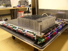
Inspired by the pin table map from X-Men, movie clip, refered to as shape display
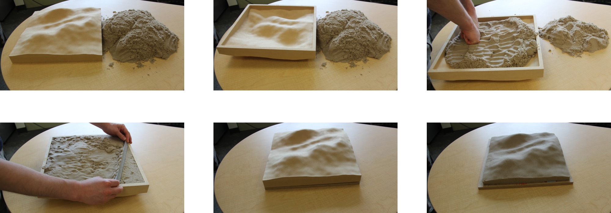
Hand sculpting from polymeric sand
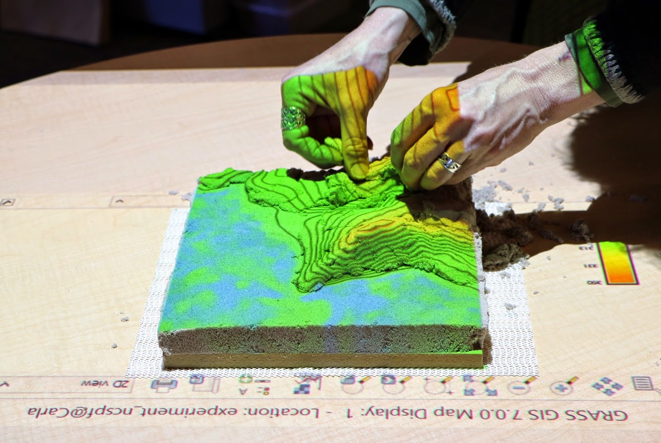
Hand sculpting with difference feedback
blue → add sand, red → remove sand3D printing
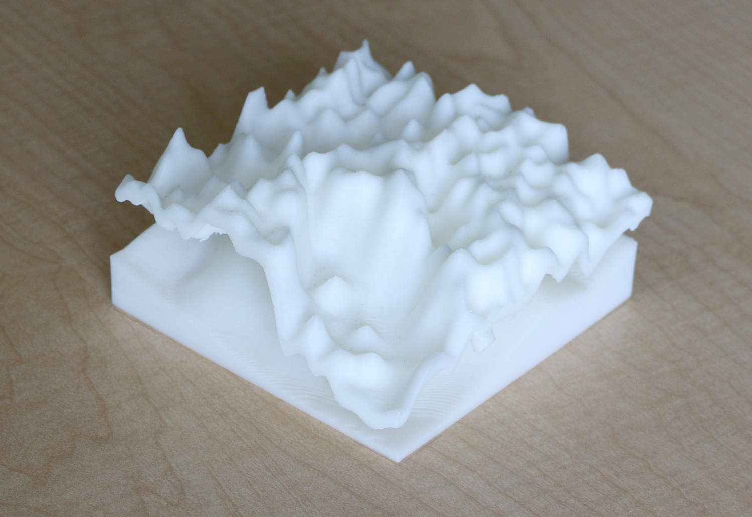
CNC routing
Large complex models and molds

Casting polymeric sand
Scale of the physical model
- scale of the model
$$s = \frac{d_m}{d_r}$$
- $s$ is the scale of the model,
- $d_m$ is the distance measured on the model,
- $d_r = (w - e)$ is the real-world distance.
- iterative process - if we want predefined scale and pre-defined (approximate) size
- what size of feature change can be detected given the resolution of the scanner (1-2mm)?
Scale of the physical model
If the smallest feature that can be reliably detected is $1 cm$ cube
- What scale the model should be to facilitate modeling dams and rivers 10m wide?
- What would be the geospatial extent of the region represented by the model size of 50 x 60 cm? how about 1 m x 80 cm ?
- If the difference in elevation in your area is 30m and you want 3 x exaggeration how high your model will be at the scale computed above for the 50 x 60 cm model?
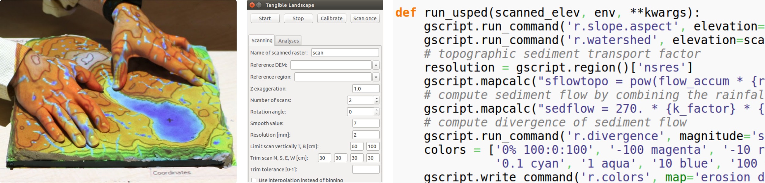
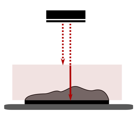
Scanning the physical model
3D sensors based on similar principles as surveying
- time of flight, near infrared laser
- stereo(photogrammetry) - overlapping images from NIR image and laser
- distortions, outliers (flying pixels), noise need to be adressed
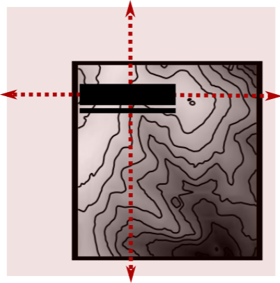
Scanning calibration
- calibration process: scanning flat surface
- tilt and radial distortion
- computing tilt angle and applying the correction to scanned point cloud
Processing the point cloud
Scanned 3D model includes all features in the scan area

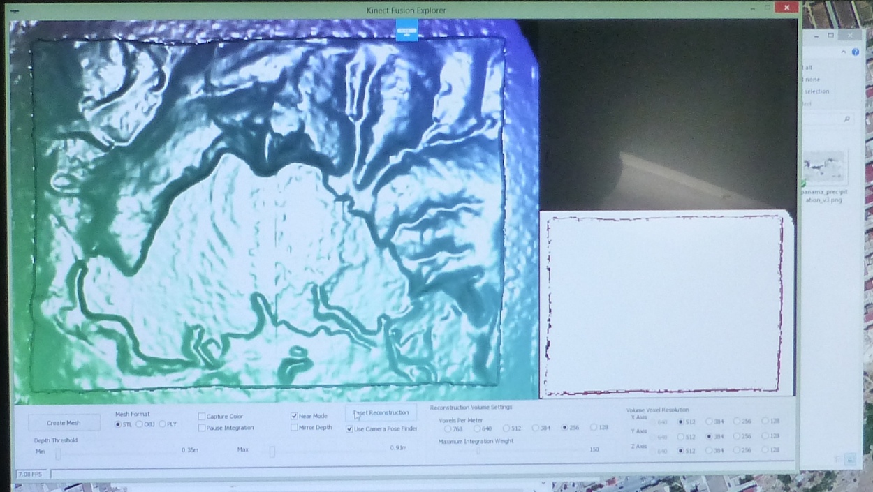
Images produced by Kinect Fusion Explorer: was the tilt filtered out here?
Processing the point cloud
- point cloud is acquired within the operator-defined horizontal and vertical extent
- flying pixels are filtered out
Processing the point cloud
Edges of the model are detected and extracted

Georeferencing - rescaling
$$
S_x = \frac{X_{east} - X_{west}}{x_{max} - x_{min}},\quad
S_y = \frac{Y_{north} - Y_{south}}{y_{max} - y_{min}},\quad
$$
$$
S_z = \frac{(S_x + S_y) / 2}{e}
$$
- $X, Y$ are DEM (real-world) coordinates,
- $x, y$ are coordinates of the physical model
- $e$ is the specified vertical exaggeration.
Georeferencing
- Transformation from the scan ("table") coordinates to the georeferenced coordinate system
Rescaling, rotation and translation
$$ G = S . R + T$$
- $S=[S_x,S_y,S_z]$ scales to real-world dimensions,
- $R$ is a rotation matrix that rotates the points around the $z$ axes by angle $\alpha$
- $T=[t_x,t_y,t_z]$ translates the points so that the lower left corner of the model matches the south-west corner of the DEM and the lowest DEM elevation matches the lowest point of the model.
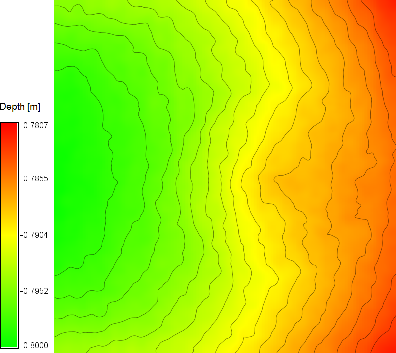
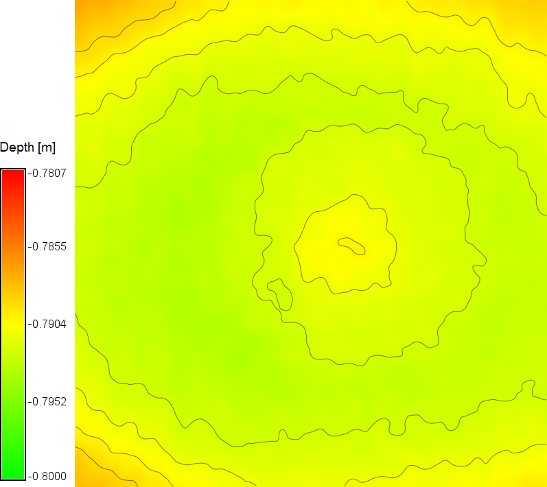
Gridding
Converting the filtered, corrected and georeferenced $(x,y,z)$ point cloud to raster
- binning: per-cell mean, nearest point
- binning: fast, but the surface is rough, with holes
- interpolation: slower, but the surface is smooth and continuous
Tangible interactions
3D scanner acquires both depth and color (RGB) information that can be used to design interactions
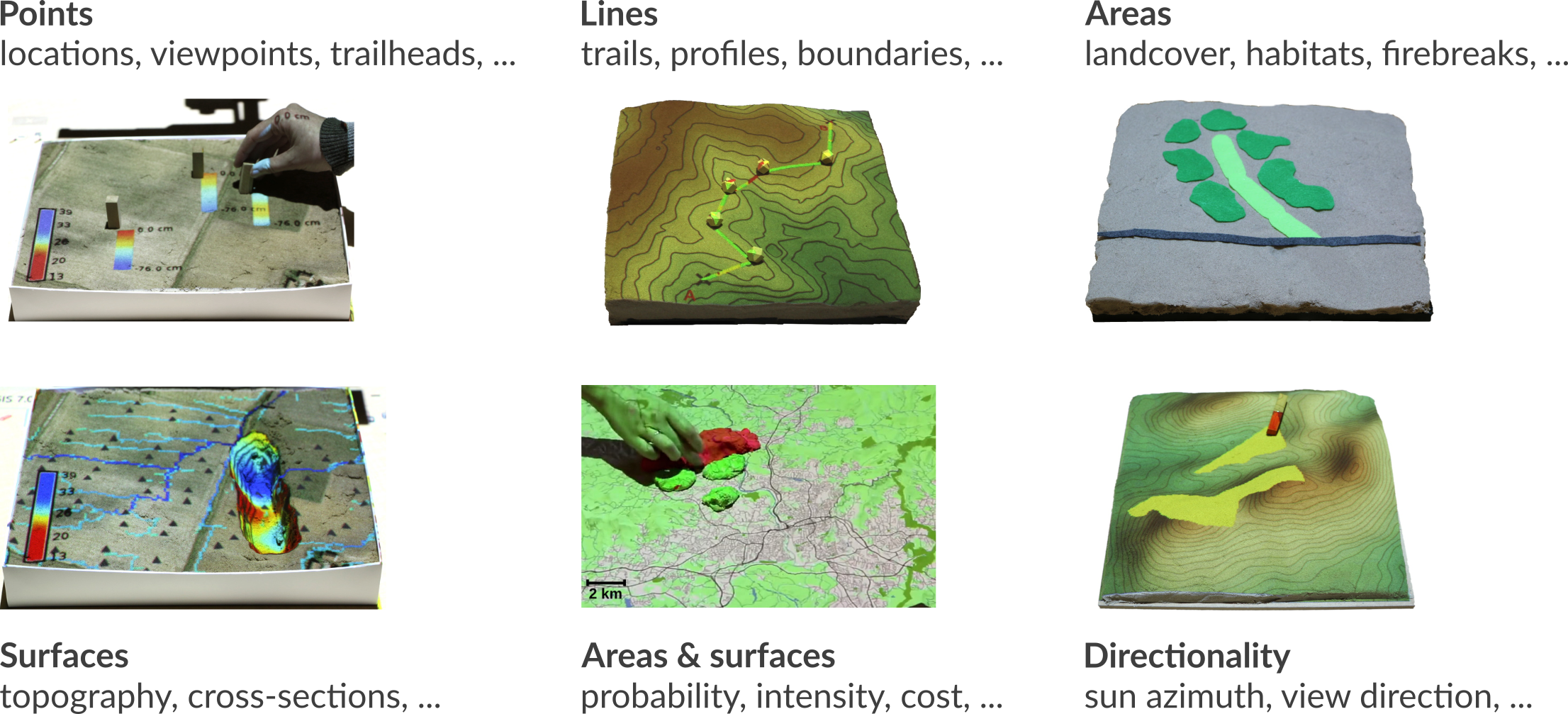
Tangible interactions: surface change
- new surface is continuously computed
- map algebra is used to detect the change if needed

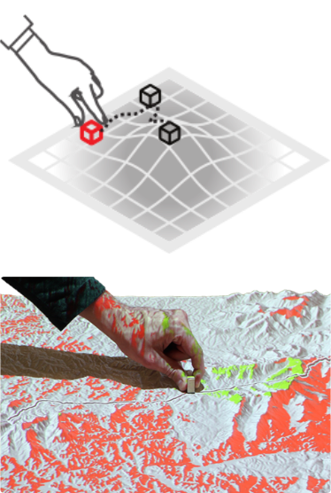
TUI: markers
- new surface is continuously computed
- map algebra is used to detect the change
- markers are identified and converted to vector point data
- vector point data can be connected into lines using TSP method
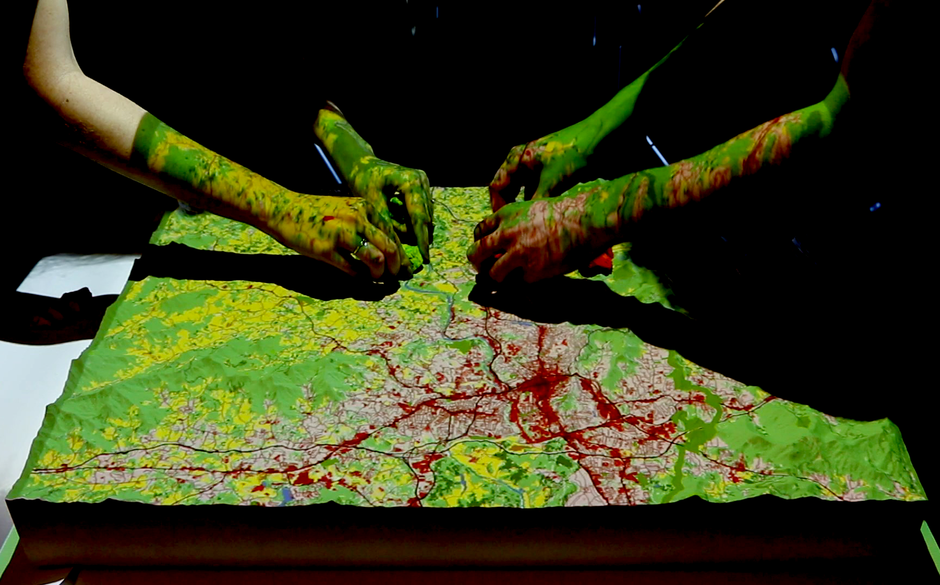
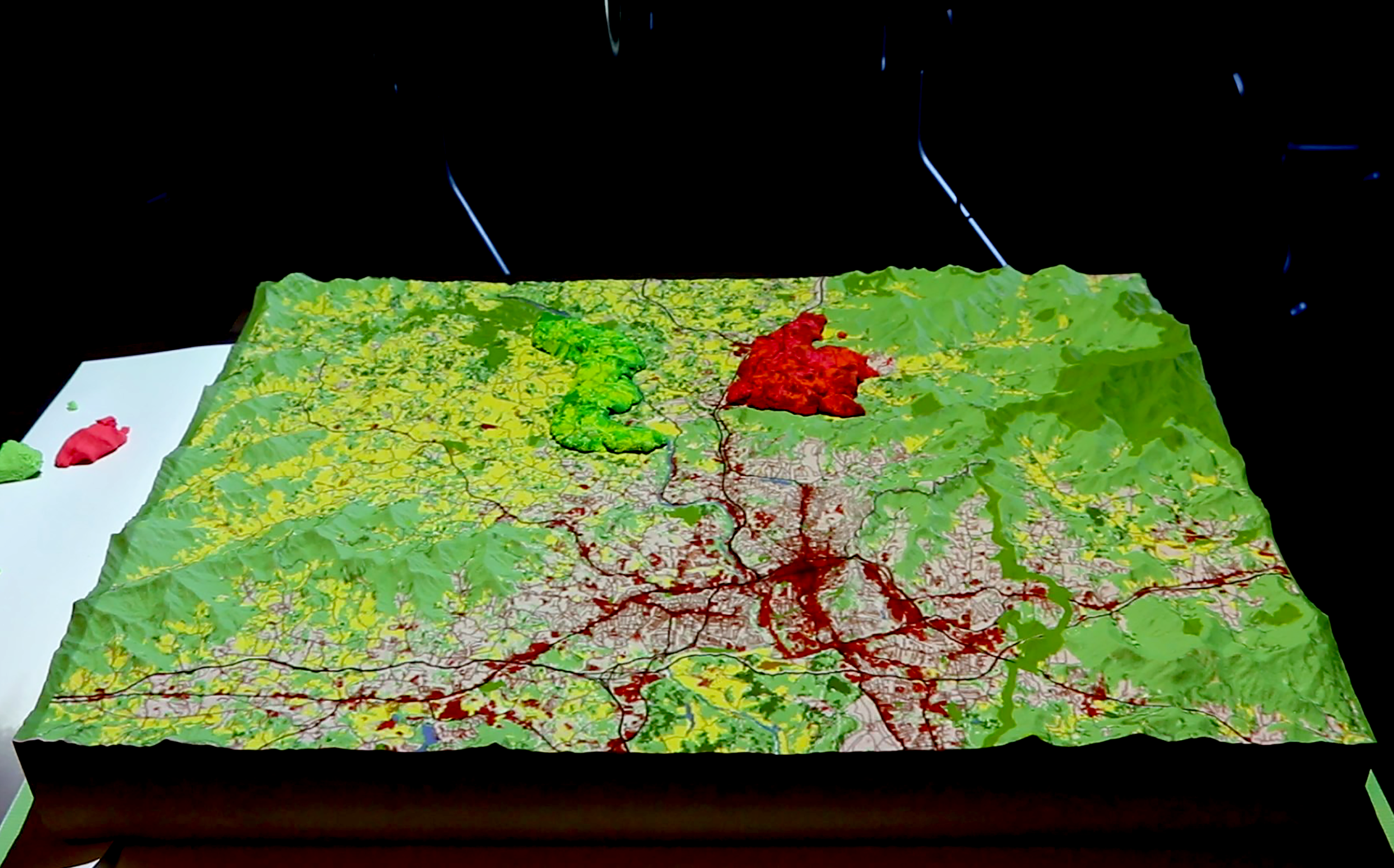
TUI: color patches
- color (RGB) data are acquired
- image segmentation and classification is used to detect the patches and assign ther attribute
- raster patches can be converted to vector polygons

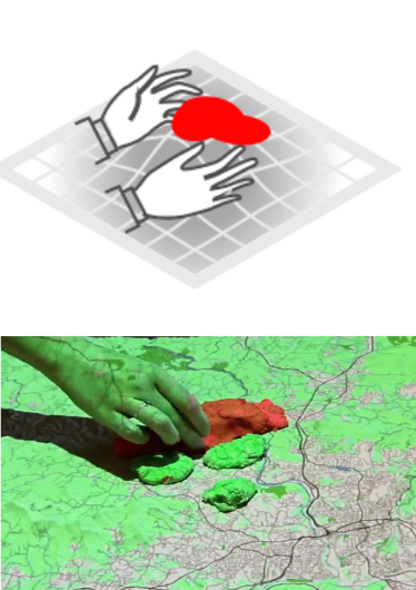
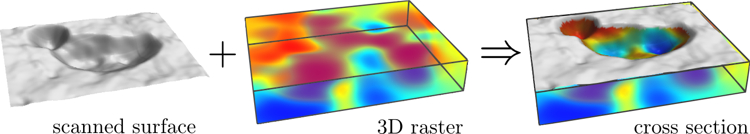
TUI: color clay
- both depth and color (RGB) data are used
- image segmentation and classification is used to detect the patches and assign ther attribute
- map algebra is used to quantify the height of the clay blob and assign related attribute
Simulations with TL
Coupling with process models to evaluate impact of scenarios
Scenarios: natural events, human modification of landscape
Visibility analysis
Visibility and line of sight
Solar radiation analysis


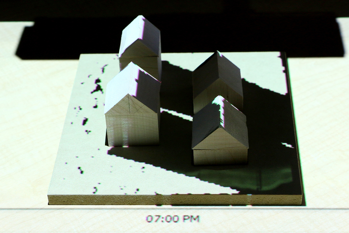
Solar irradiation and cast shadows
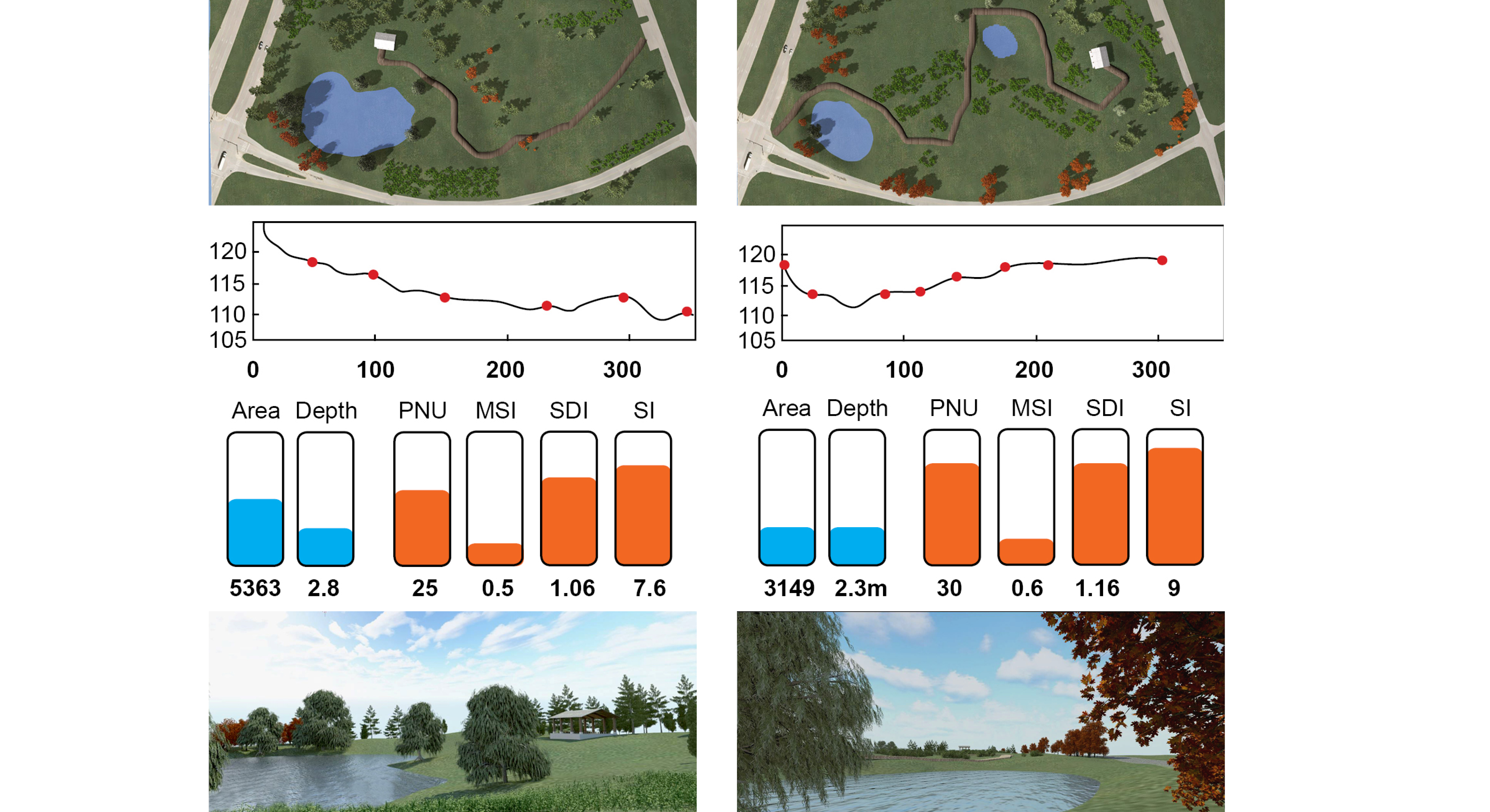
Trail planning
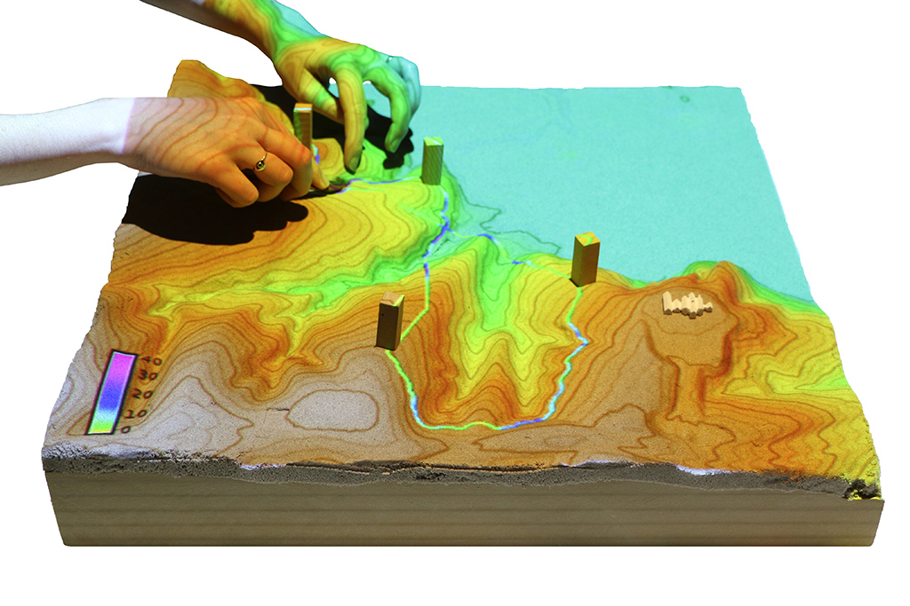
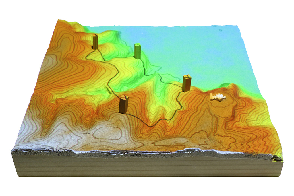
Optimized trail routing between waypoints based on energetics, topography, and cost maps with feedback including trail slopes and viewsheds
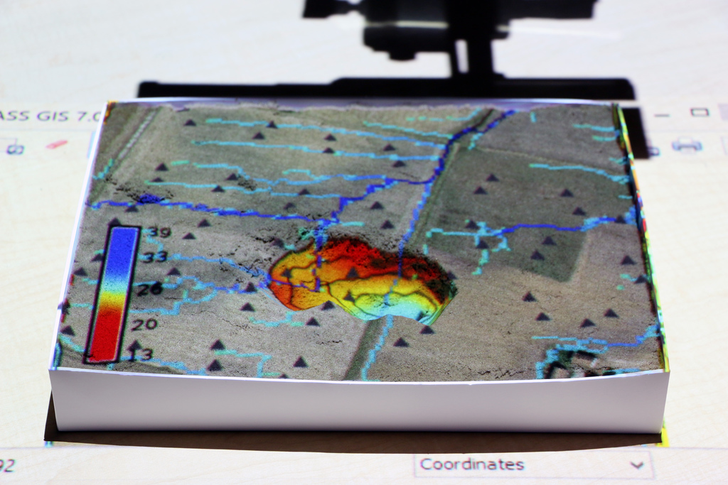
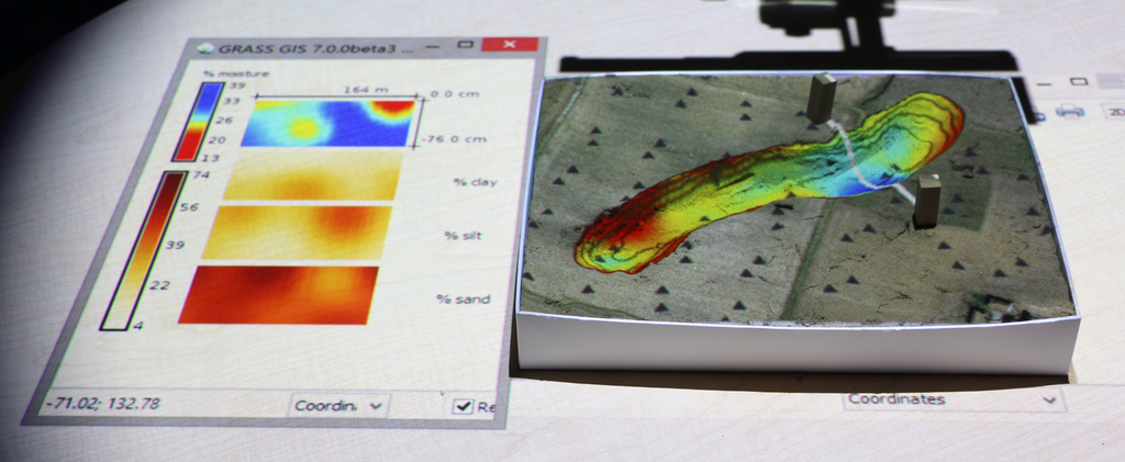
3D soil moisture exploration

Dam breach
Applications: wildfire spread
Management of infectious disease
- Sudden Oak Death (SOD)
- simulating disease using spatially-explicit model
- workshop with expert stakeholders

Urban growth
Simulation of urban growth scenarios with FUTURES model
Meentemeyer, et al. (2013), FUTURES: multilevel simulations of emerging urban–rural landscape structure using a stochastic patch-growing algorithm.
Serious games: Termite infestation
Manage the spread of termites across a city by treating city blocks using a model of biological invasion in R

Serious games: coastal flooding

Save houses from coastal flooding by building coastal defenses (Bald Head Island, NC)
Structured problem-solving with rules, challenging objectives, and scoring
Florence hurricane flooding
Realtime 3D rendering with Blender

Designing with Tangible Landscape
Open source Tangible Landscape
- TL plugin for GRASS GIS
github.com/tangible-landscape/grass-tangible-landscape - GRASS GIS module for importing data from Kinect v2
github.com/tangible-landscape/r.in.kinect - TL repository on Open Science Framework osf.io/w8nr6
- TL website: tangible-landscape.github.io
- TL wiki:
github.com/tangible-landscape/grass-tangible-landscape/wiki
Resources
- Book: Petrasova et al., 2018, Tangible Modeling with Open Source GIS, second edition, Springer Int. Pub.