Photogrammetry and Structure from Motion Concepts

Center for Geospatial Analytics at North Carolina State University

Corey White adapted from Justyna Jeziorska and Helena Mitasova

Objectives

  • Distinguish remote sensing from photogrammetry and explain what each contributes to UAS mapping
  • Explain why a raw aerial photograph cannot be measured like a map, and what orthorectification fixes
  • Describe how Structure from Motion (SfM) recovers 3D geometry from overlapping 2D images
  • Explain how geotags, ground control points, and RTK/PPK positioning anchor a model to the ground
  • Recognize the imaging conditions that make SfM succeed or fail

From photographs to measurements

Where this lecture sits

The course pipeline: rules and regulations, plan the flight, collect imagery, SfM processing (highlighted), GIS analytics, with the topic that covers each step

Why processing before planning? You cannot plan a flight well until you know what the processing needs from the imagery

Remote sensing and photogrammetry

flowchart TB
    IMG["Aerial and UAS images"]
    RS["Remote sensing<br/>What is it?<br/>land cover, vegetation, temperature"]
    PG["Photogrammetry<br/>Where is it, how big is it?<br/>position, shape, elevation"]
    GIS["GIS<br/>analysis, data fusion, maps"]
    IMG --> RS
    IMG --> PG
    RS --> GIS
    PG --> GIS
    style PG fill:#006600,stroke:#006600,color:#ffffff

Passive and active sensing

Passive sensors (RGB, multispectral, thermal cameras) record reflected or emitted energy; depth is not measured, it is inferred from parallax between overlapping images

Active sensors (lidar, radar) emit energy and measure the return; range is measured directly

This topic: passive RGB imagery, with 3D inferred by Structure from Motion

A short history

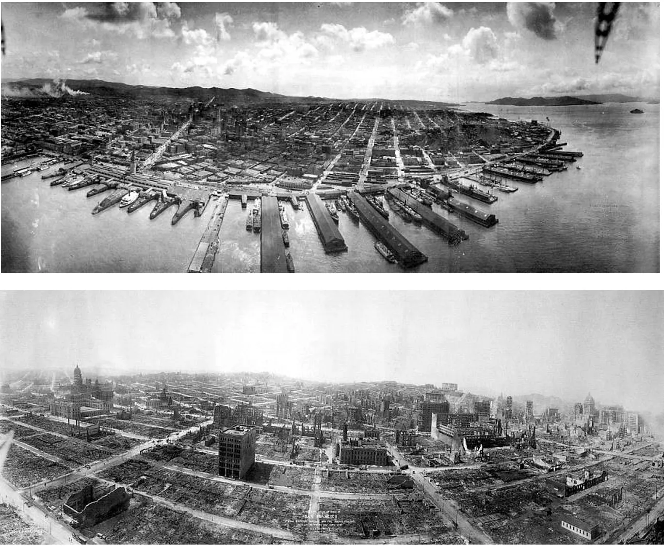
Two panoramic kite photographs of San Francisco in 1906 showing the waterfront and the burned city

San Francisco after the 1906 earthquake, from a kite (George Lawrence)

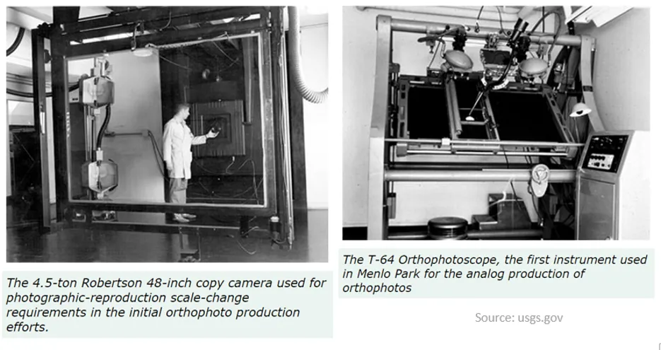
Two black and white photographs of room-sized analog orthophoto instruments at USGS

Analog orthophoto production at USGS: a 4.5-ton copy camera and the T-64 Orthophotoscope
  • 1850s: first aerial photographs from balloons; kites and pigeons follow
  • 1900s to 1940s: aerial survey cameras, stereoplotters, wartime mapping
  • 1960s to 1990s: analog orthophoto instruments, then analytical plotters
  • 2000s onward: digital cameras, computer vision, and SfM on consumer hardware

Then and now

Analog photogrammetry: calibrated metric cameras, film, stereoplotters, manual point measurement by trained operators

Structure from Motion: consumer cameras, automatic feature matching, self-calibration, thousands of images processed on a laptop

Digital photogrammetry: scanned or digital imagery, analytical solutions, still needs camera calibration and manual control measurement
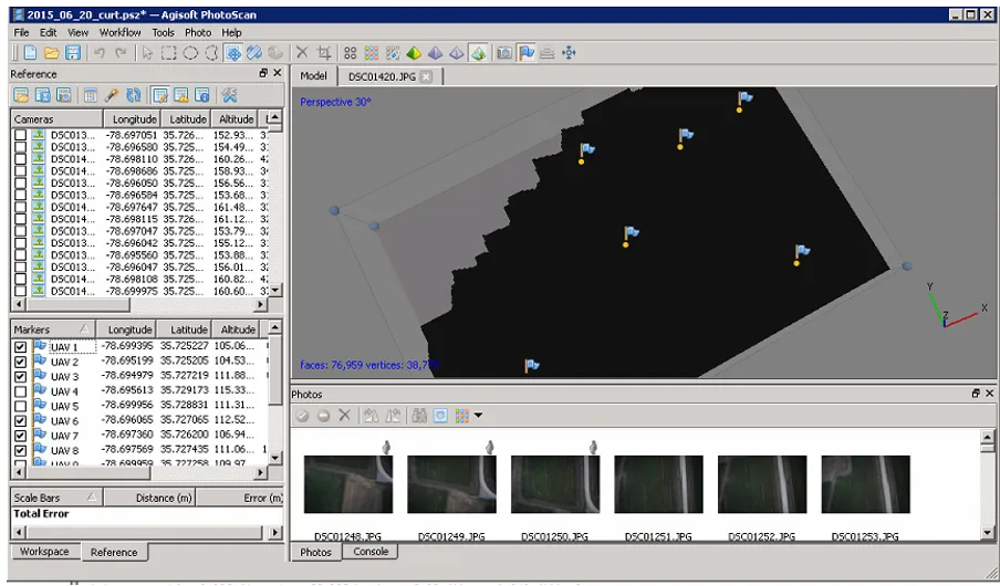
Screenshot of photogrammetry software with a camera list, ground control markers, model view, and photo strip

Camera positions, ground control markers, and photos in an SfM project

Types of aerial imagery

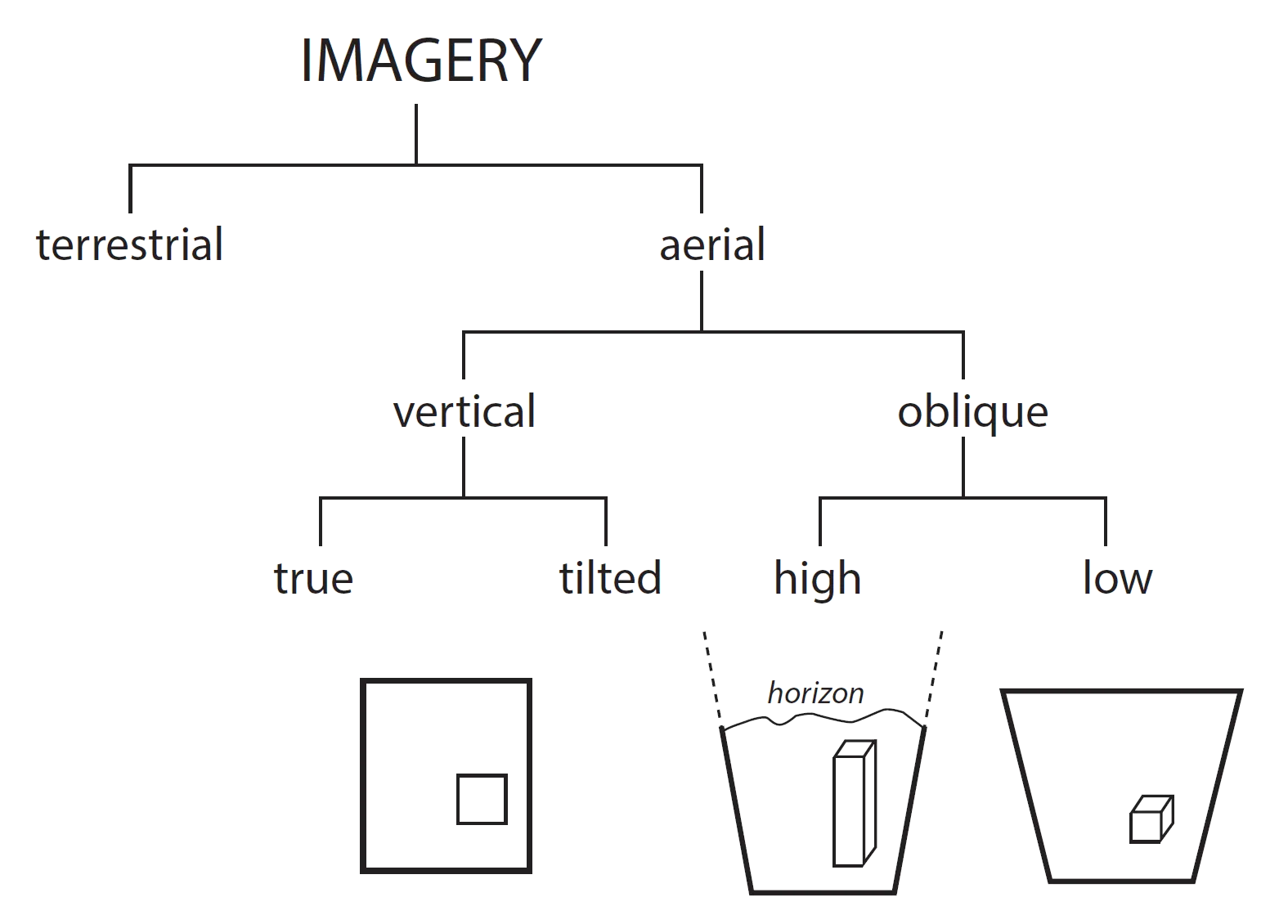
Tree diagram classifying imagery as terrestrial or aerial, aerial as vertical or oblique, with sketches of each view

Vertical (nadir) Oblique
Camera Pointing straight down Tilted; high oblique shows the horizon
Scale Nearly uniform Varies across the frame
Good for Orthophotos, DSMs, measurement Facades, undercuts, 3D texture, context
Mapping flights The default Added to nadir for buildings and steep terrain

Why a photograph is not a map

Camera geometry

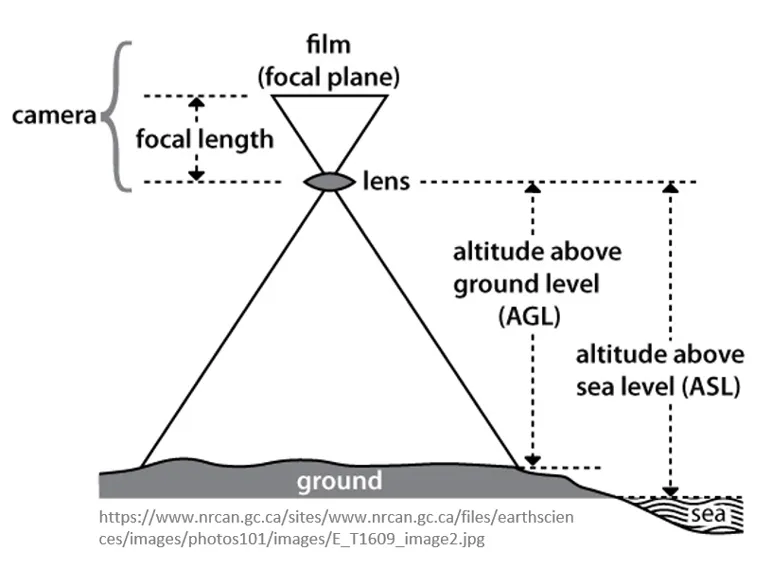
Diagram of a camera with focal length between lens and film, and altitude above ground level and above sea level

Source: Natural Resources Canada

Focal length: distance from the lens to the sensor; with sensor size it sets the field of view

Flying height (AGL): altitude above the ground, not above sea level; with focal length it sets image scale

Ground sampling distance (GSD): the ground size of one pixel; the resolution of your final products. The formula and how to plan for it come in Topic 3

Perspective versus orthographic
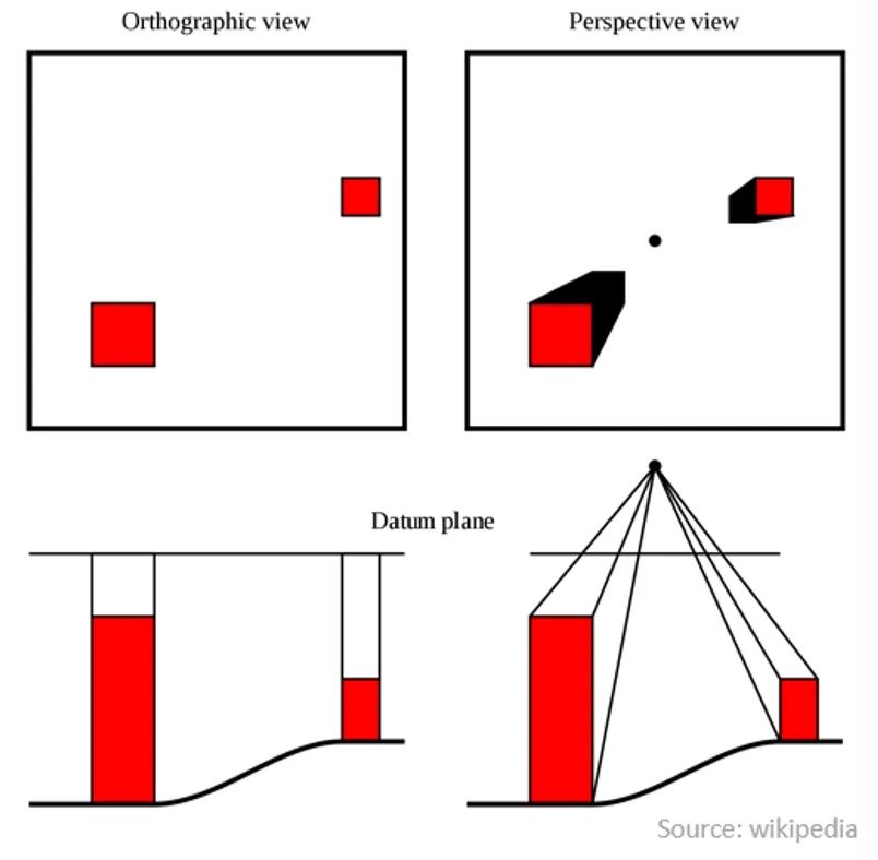
Two blocks at different heights shown in orthographic view at true position and in perspective view displaced outward

Source: Wikipedia
  • A camera is a perspective projection: all rays pass through one point, the lens
  • A map is an orthographic projection: every point is projected straight down
  • In a perspective image, anything above the datum plane is displaced outward from the image center, and the higher it is the more it moves

Relief displacement
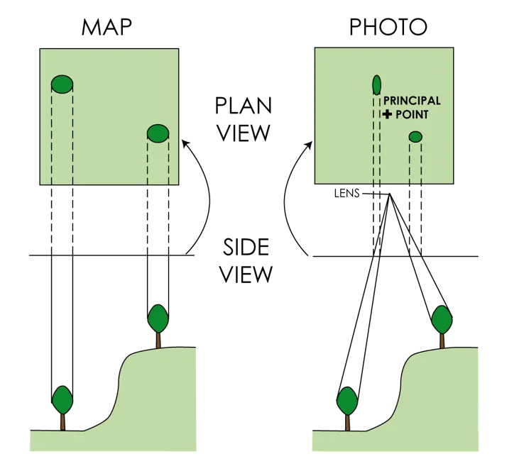
Map and photo of two trees on a slope, showing their positions shift in the photo relative to the map

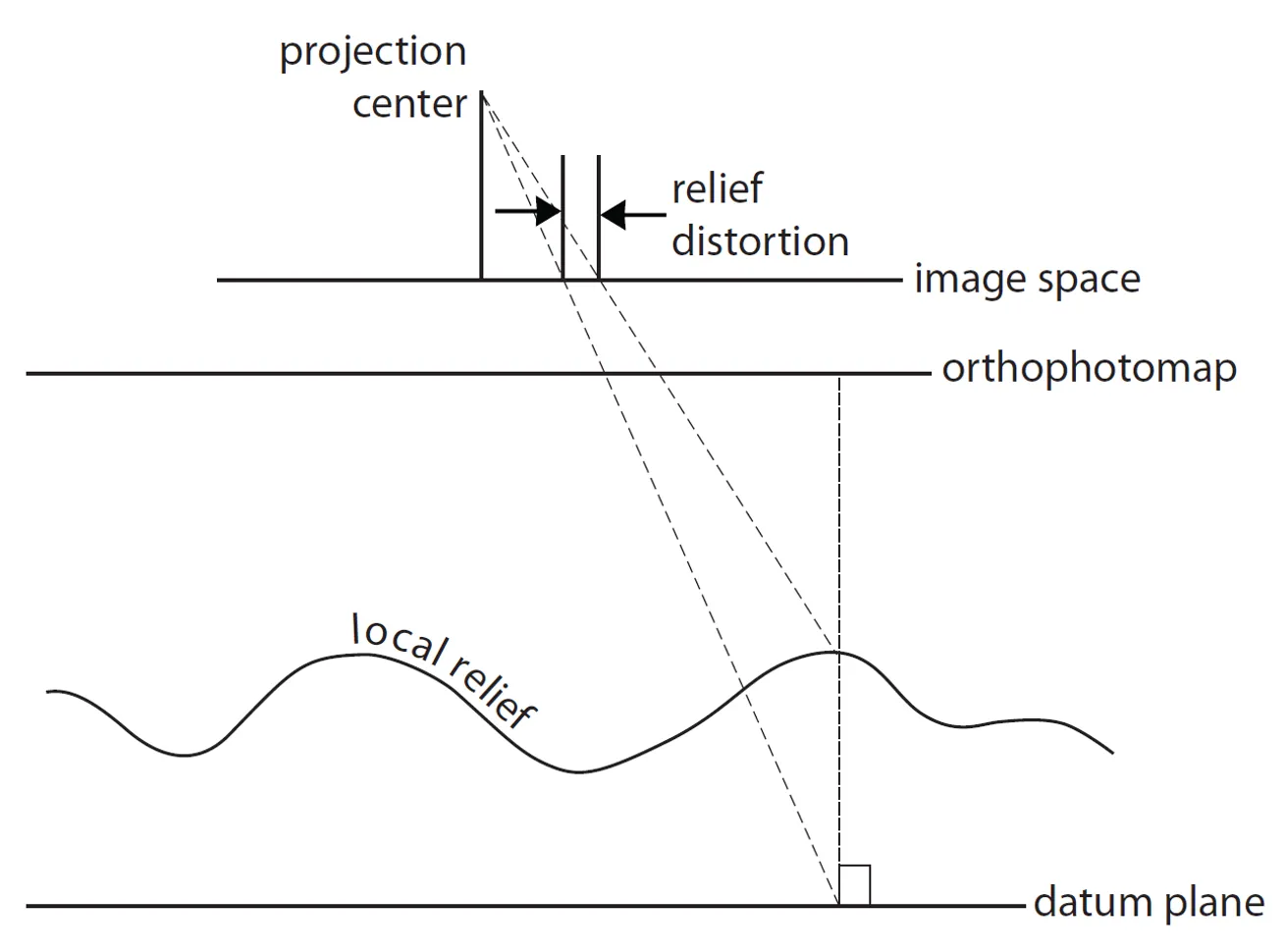
Cross section showing a ray from the projection center through relief to the datum plane and the resulting relief distortion on the image

Relief displacement: the shift of an image point caused by the elevation of the ground point, radially away from the principal point

Other sources of distortion

Source Effect Remedy
Camera tilt Scale varies across the frame Gimbal, exterior orientation solved in processing
Lens distortion Straight lines bow (radial), image shears (tangential) Camera calibration, self-calibration in SfM
Rolling shutter Rows exposed at different times; features smear in motion Global shutter, slower flight, rolling shutter model
Terrain relief Radial displacement (previous slide) Surface model and orthorectification

Orthorectification

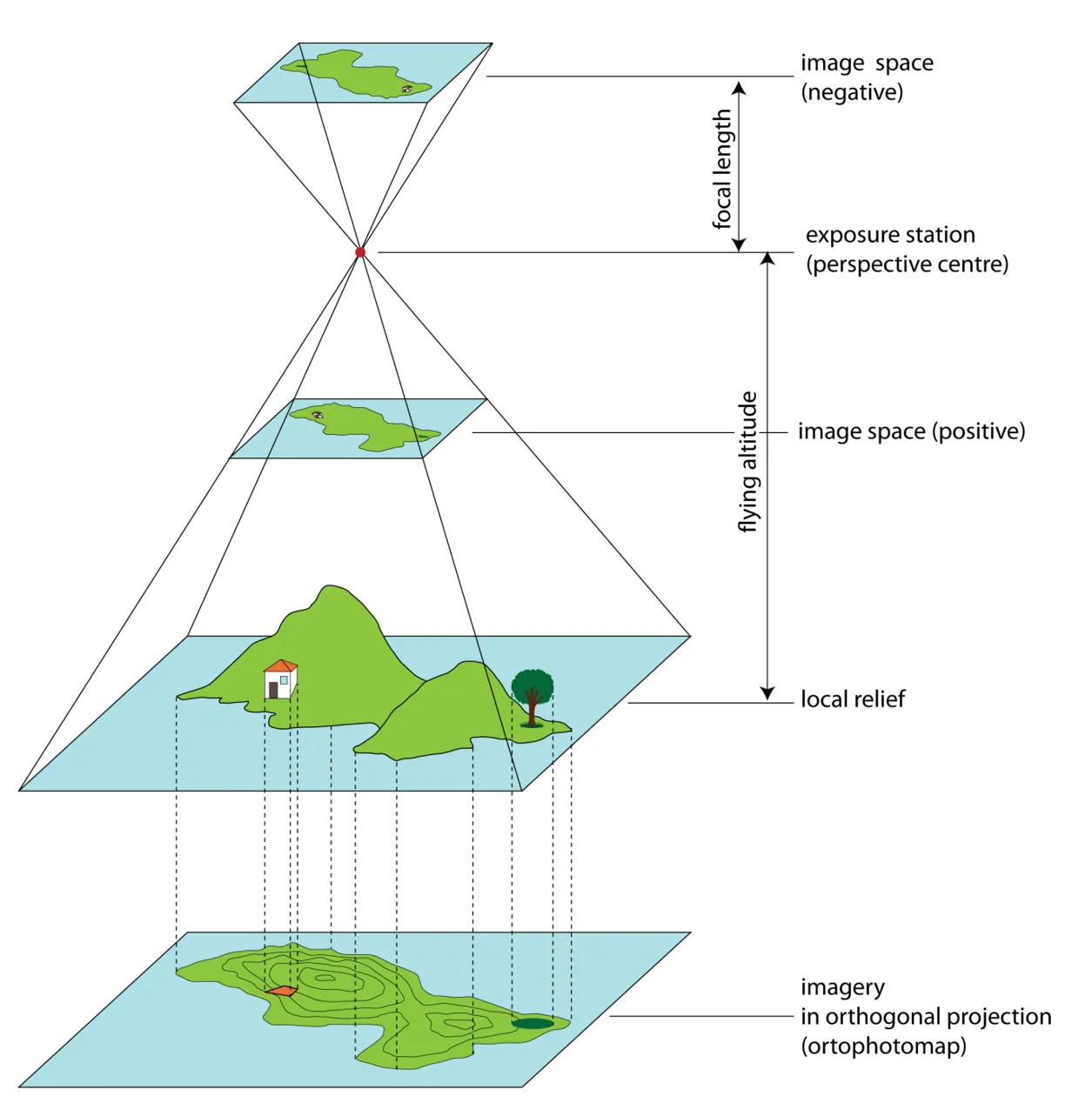
Diagram of image space, exposure station, terrain with relief, and the orthophotomap below it in orthogonal projection

Orthorectification re-projects each image pixel from the camera’s perspective onto a map plane. It needs:

  1. The camera model (interior orientation: focal length, principal point, lens distortion)
  2. The camera position and attitude for every photo (exterior orientation)
  3. A surface model of the terrain (and, for a true orthophoto, of buildings and trees)

Output: an orthophoto, a photograph with the geometry of a map

The orthophoto
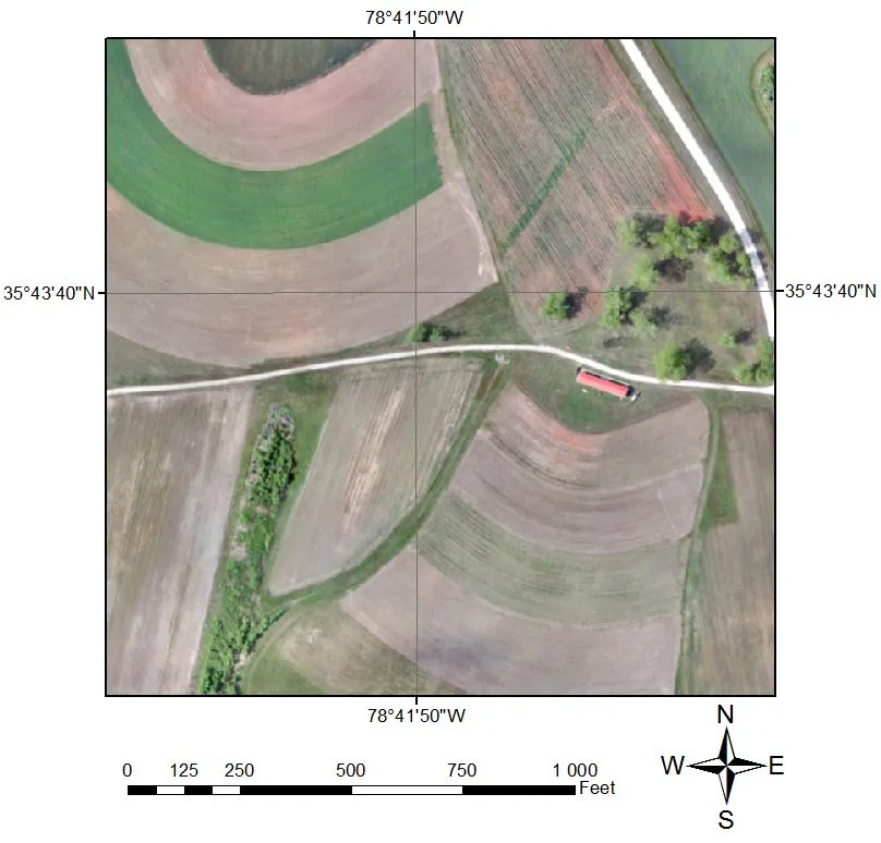
UAS orthophoto of fields and a road with a latitude longitude grid, scale bar, and north arrow

UAS orthophoto with a coordinate grid and scale bar
  • Uniform scale: distances, areas, and angles are measurable
  • Georeferenced: every pixel has a map coordinate
  • An RGB raster like any other; loads into GIS as a basemap or analysis layer
  • Its accuracy is only as good as the surface model and control behind it
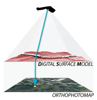
Camera above a digital surface model projecting down to an orthophotomap

How SfM recovers 3D from 2D

It starts with overlap

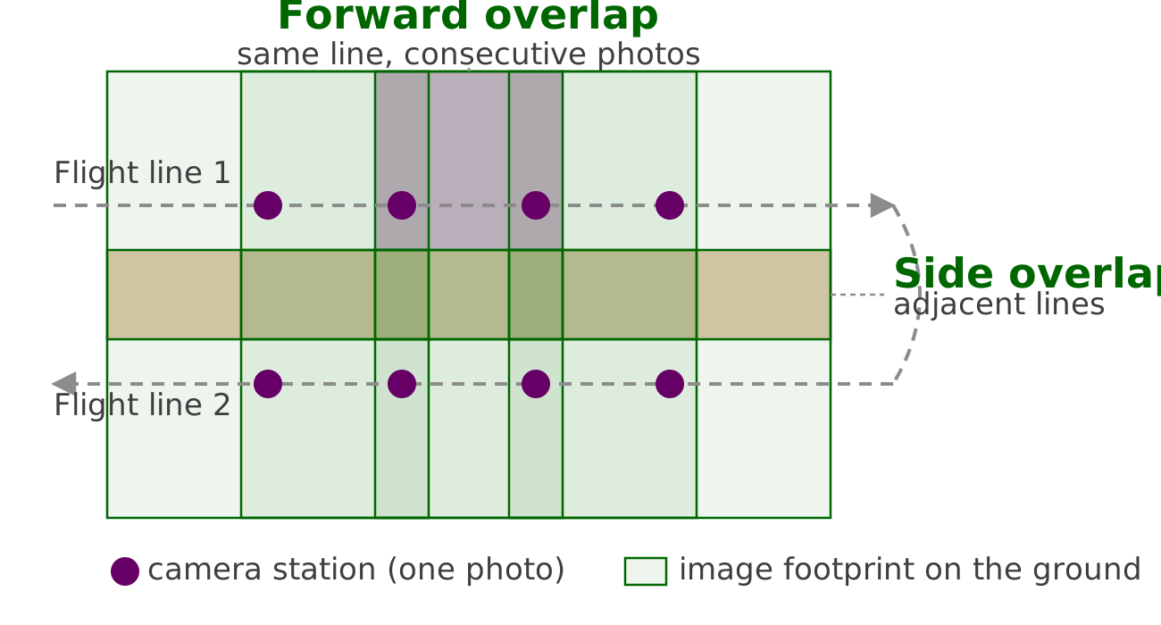
Two flight lines with overlapping image footprints; the forward overlap band between consecutive photos and the side overlap band between lines are shaded

Two flight lines of a lawnmower pattern with the forward and side overlap bands shaded
Overlap Typical for SfM
Forward (along the line) 75 to 85%
Side (between lines) 60 to 80%

Why so much? Every ground point must appear in at least 3 images, ideally 5 or more, for its 3D position to be solved reliably

Parallax: the shift of a feature between photos taken from different positions; it is what makes depth recoverable. Classical stereo used one pair per point; SfM wants many

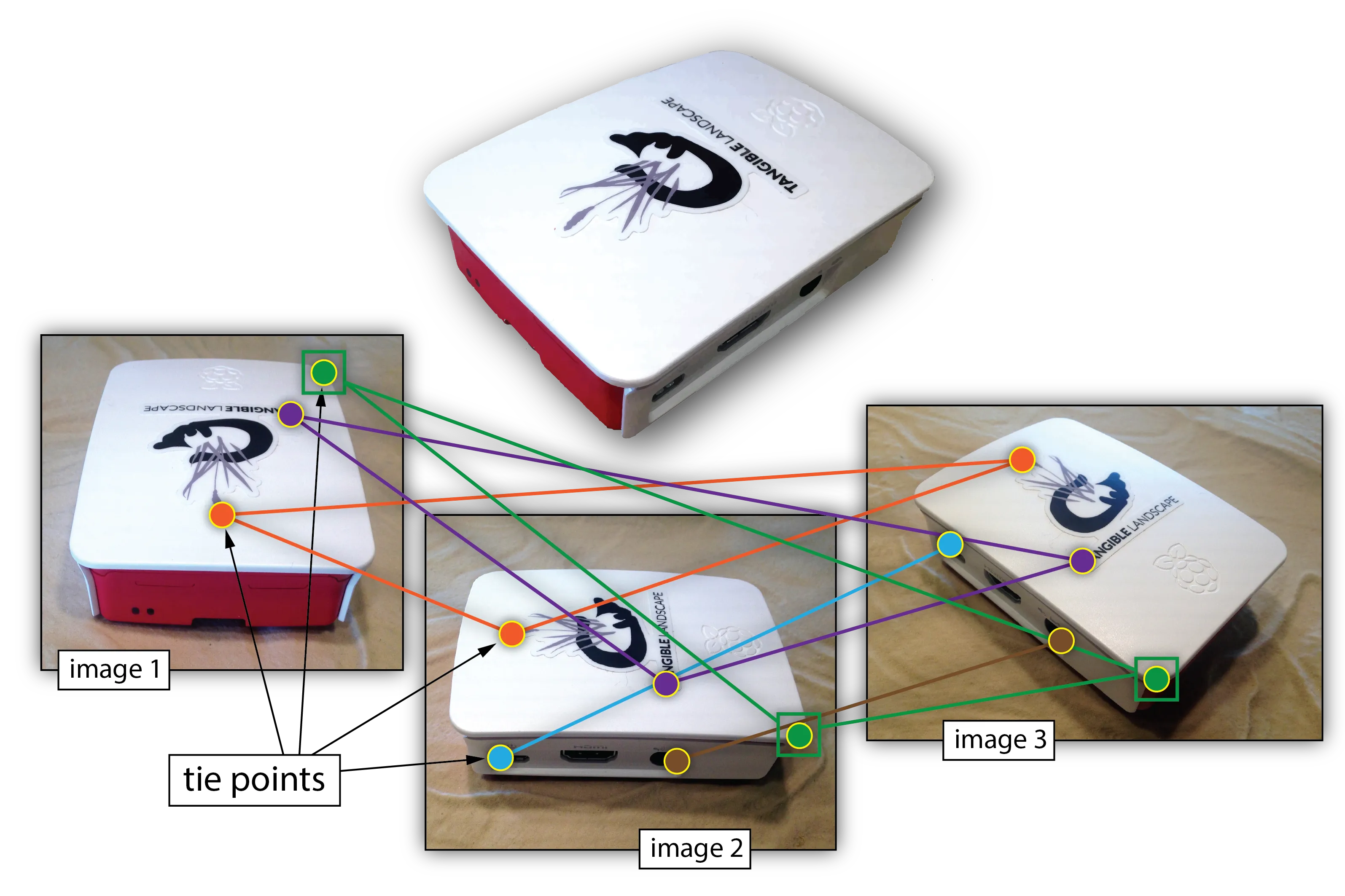
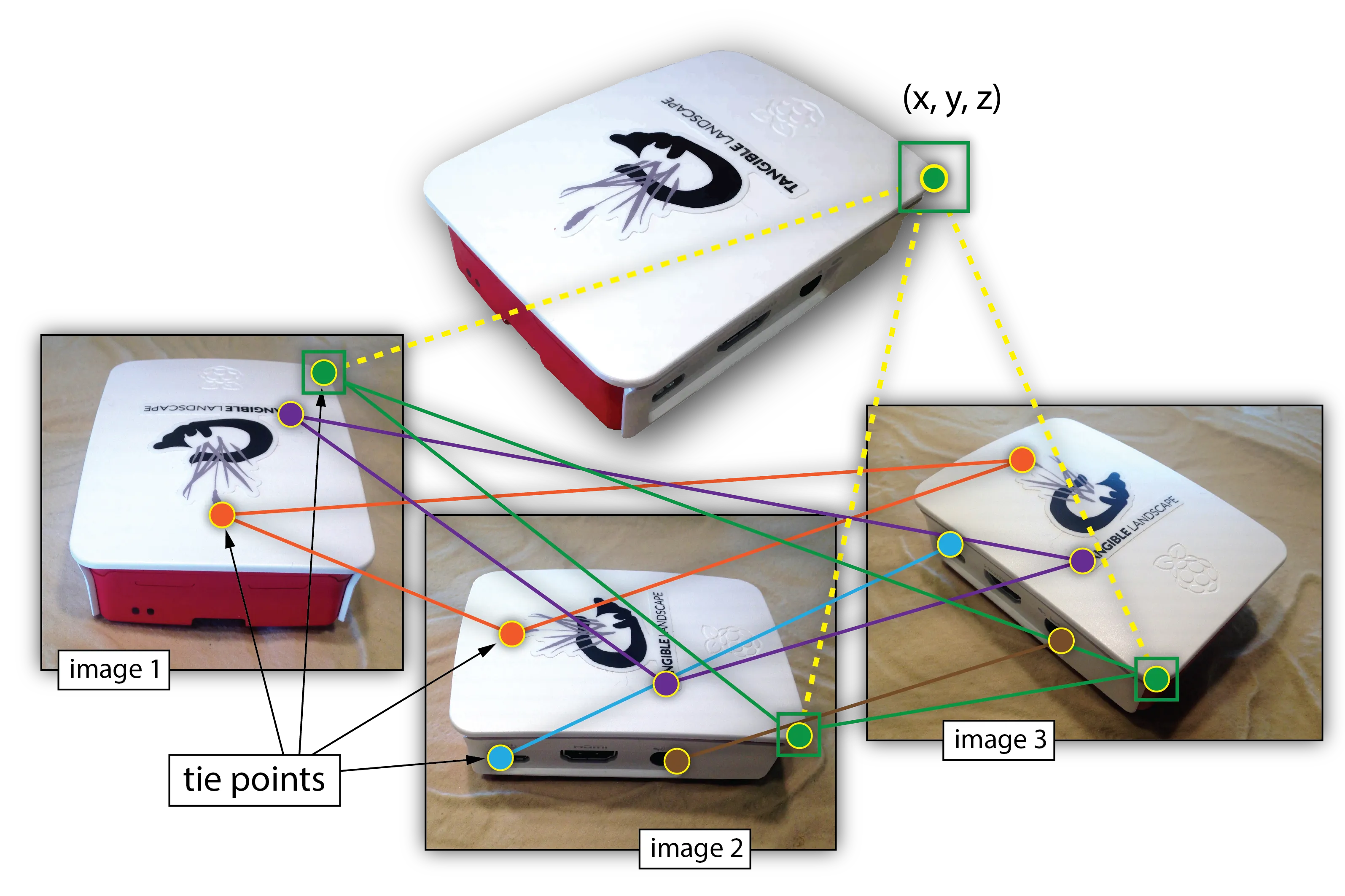
Tie points: the desk-scale version
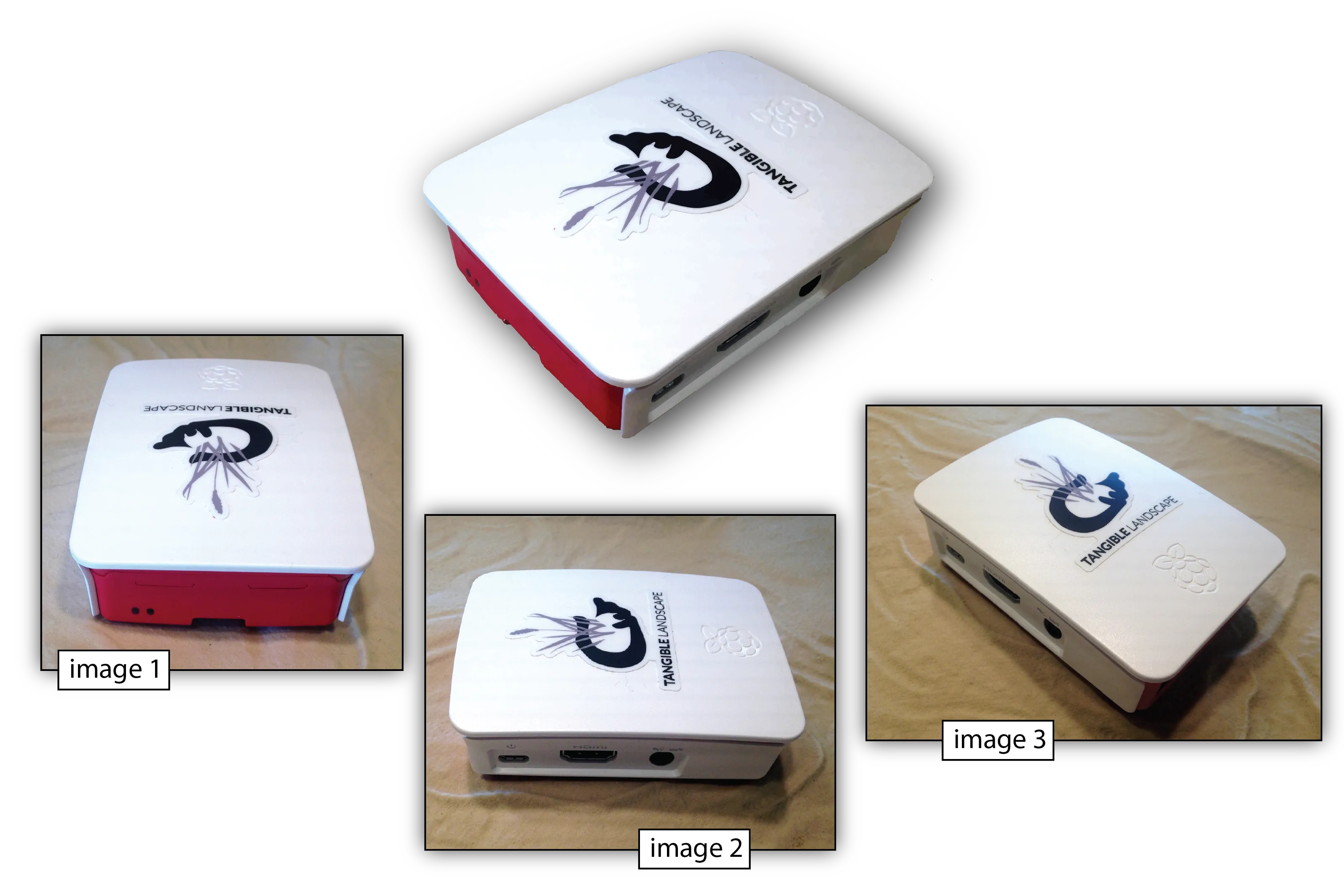
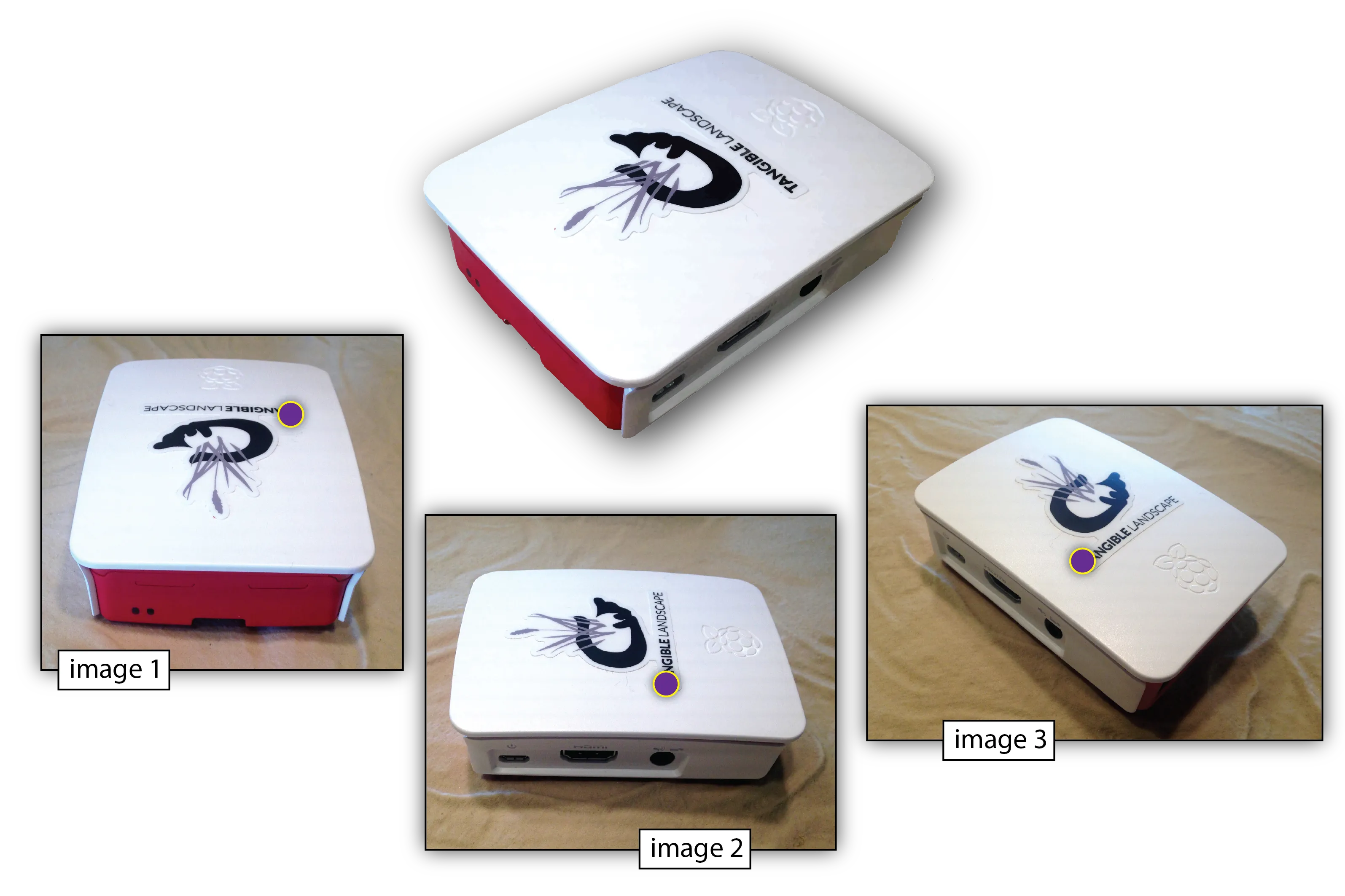
Three photographs of a small box taken from different positions

The same three photographs with one feature marked in each

Colored lines connecting matched tie points across the three photographs

Rays from the three photographs intersecting at one reconstructed 3D point on the box

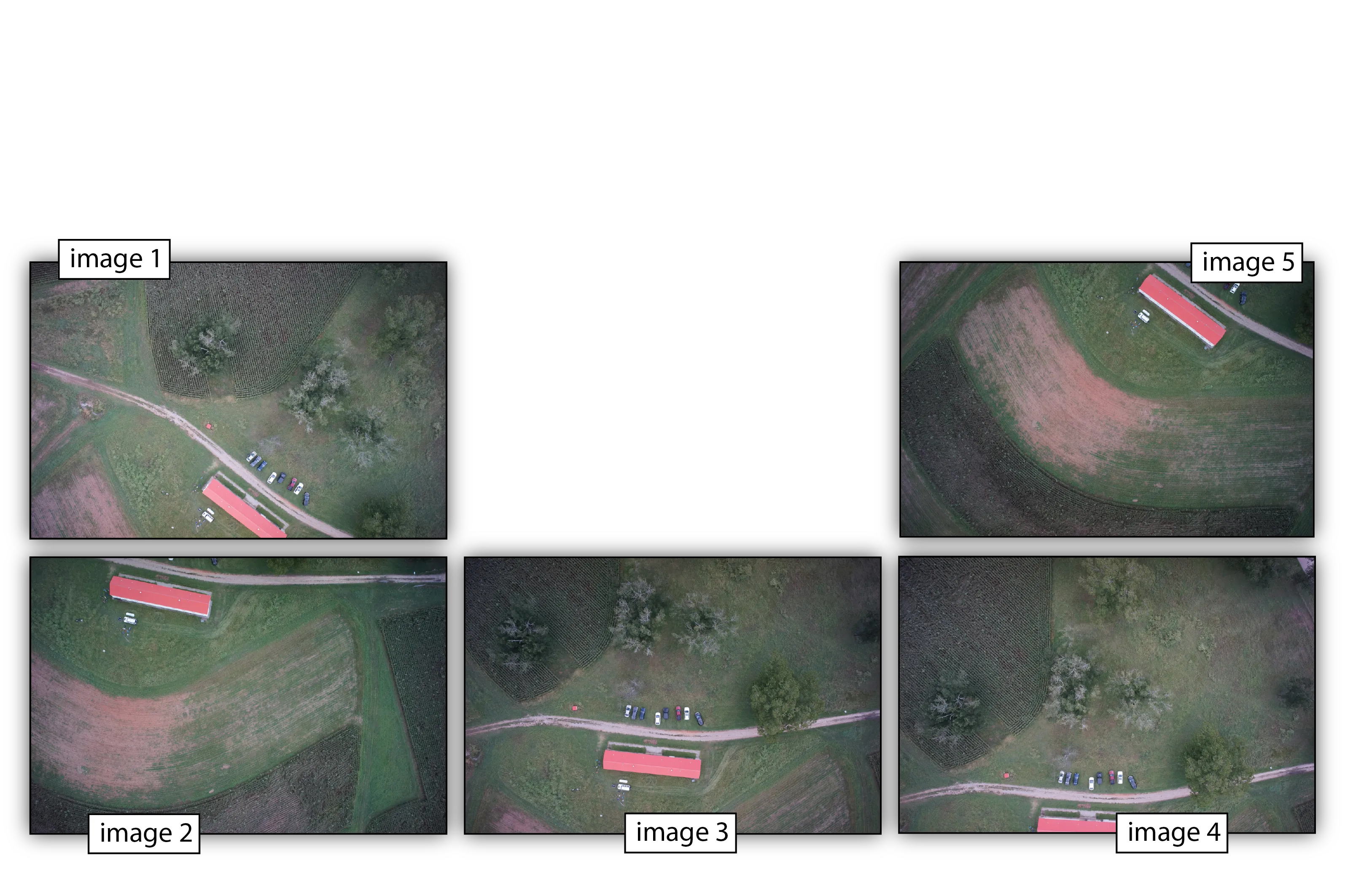
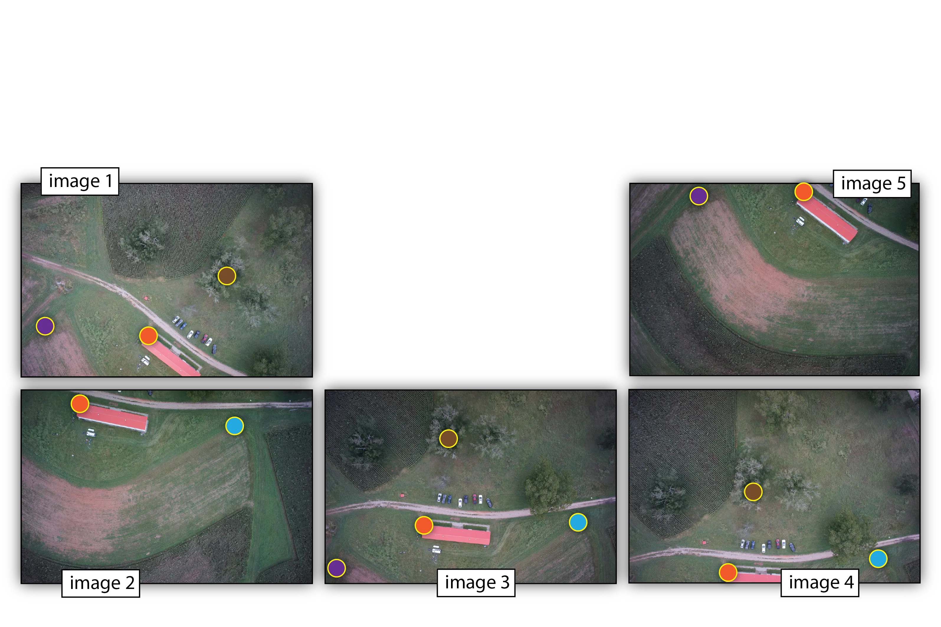
Tie points: the aerial version

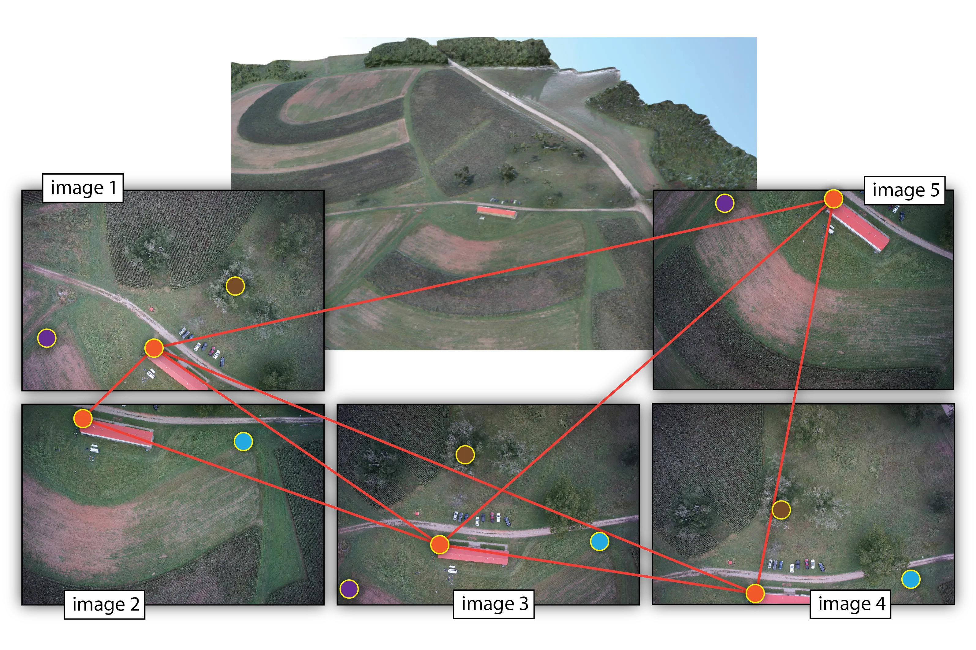
Five overlapping nadir drone images of a field with a red-roofed shed

The five drone images with matching features marked in each

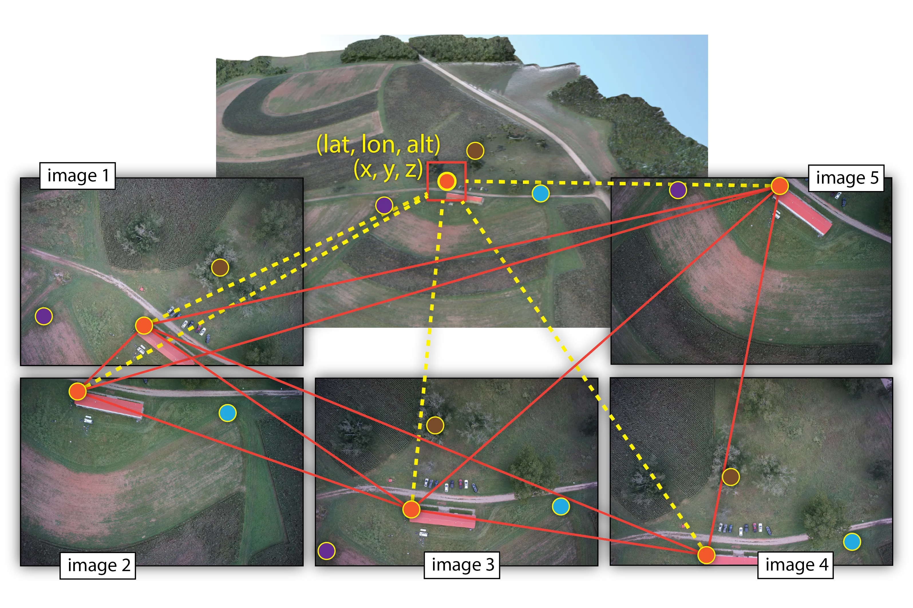
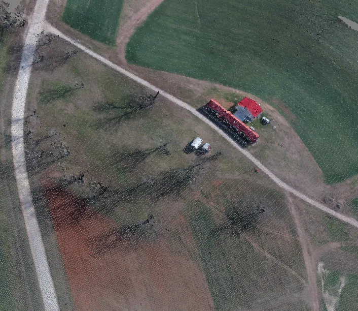
Matched features connected across the five drone images below a reconstructed 3D view of the site

Rays from the five drone images intersecting at one reconstructed point on the 3D model of the site

SfM at work

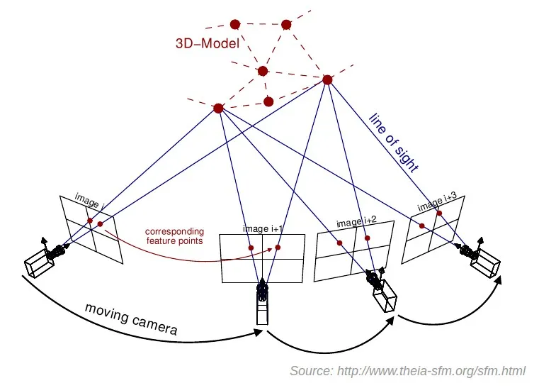
Multiple-view geometry

A moving camera captures a sequence of images; lines of sight to corresponding feature points intersect at a 3D model

Source: theia-sfm.org

SfM solves three linked questions at once:

Correspondence: which pixels in different images show the same point?

Structure: given the matches, where are those points in 3D?

Motion: where was the camera, and how was it oriented, for every image?

Bundle adjustment

Reprojection error: how far each 3D point lands from its detected tie point when projected back into the image; the quantity being minimized

Exterior orientation: position (X, Y, Z) and attitude (omega, phi, kappa) of every camera, solved for all images together

Interior orientation: focal length, principal point, and lens distortion, self-calibrated from the images

  • A non-linear least-squares optimization over every camera and every tie point
  • Outputs: refined camera poses, a sparse point cloud, and a camera model
  • Weak geometry (little overlap, low texture, one flying height) leaves the solution poorly constrained
  • Lecture 2B looks at the Metashape settings that control it

From tie points to products

Stage Input Output
Feature detection and matching Overlapping images Tie points
Bundle adjustment (alignment) Tie points, initial camera positions Camera poses, camera model, sparse point cloud
Dense matching (multi-view stereo) Aligned images Depth maps, dense point cloud
Surface reconstruction Dense cloud Mesh and DSM
Orthorectification and mosaicking Images, camera poses, DSM Orthophoto

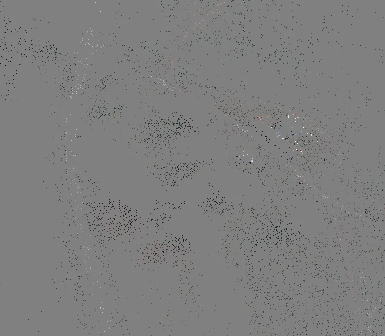
Sparse point cloud of a field, scattered points on a grey background

Sparse cloud

Dense point cloud of the same field showing the road, trees, and shed

Dense cloud

Anchoring the model to the ground

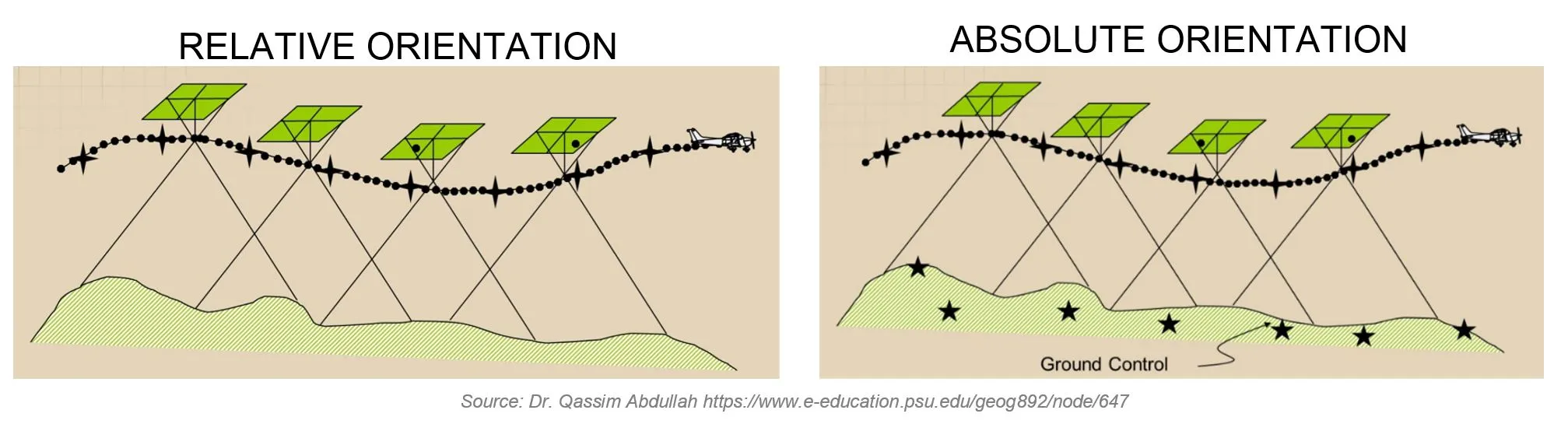
Relative and absolute orientation

Left: images fitted to each other above terrain; right: the same block fitted to ground control points marked by stars

Source: Dr. Qassim Abdullah, Penn State GEOG 892

  • Relative orientation: images fit each other.
  • Absolute orientation: the block fits the ground, through ground control or accurately known camera positions

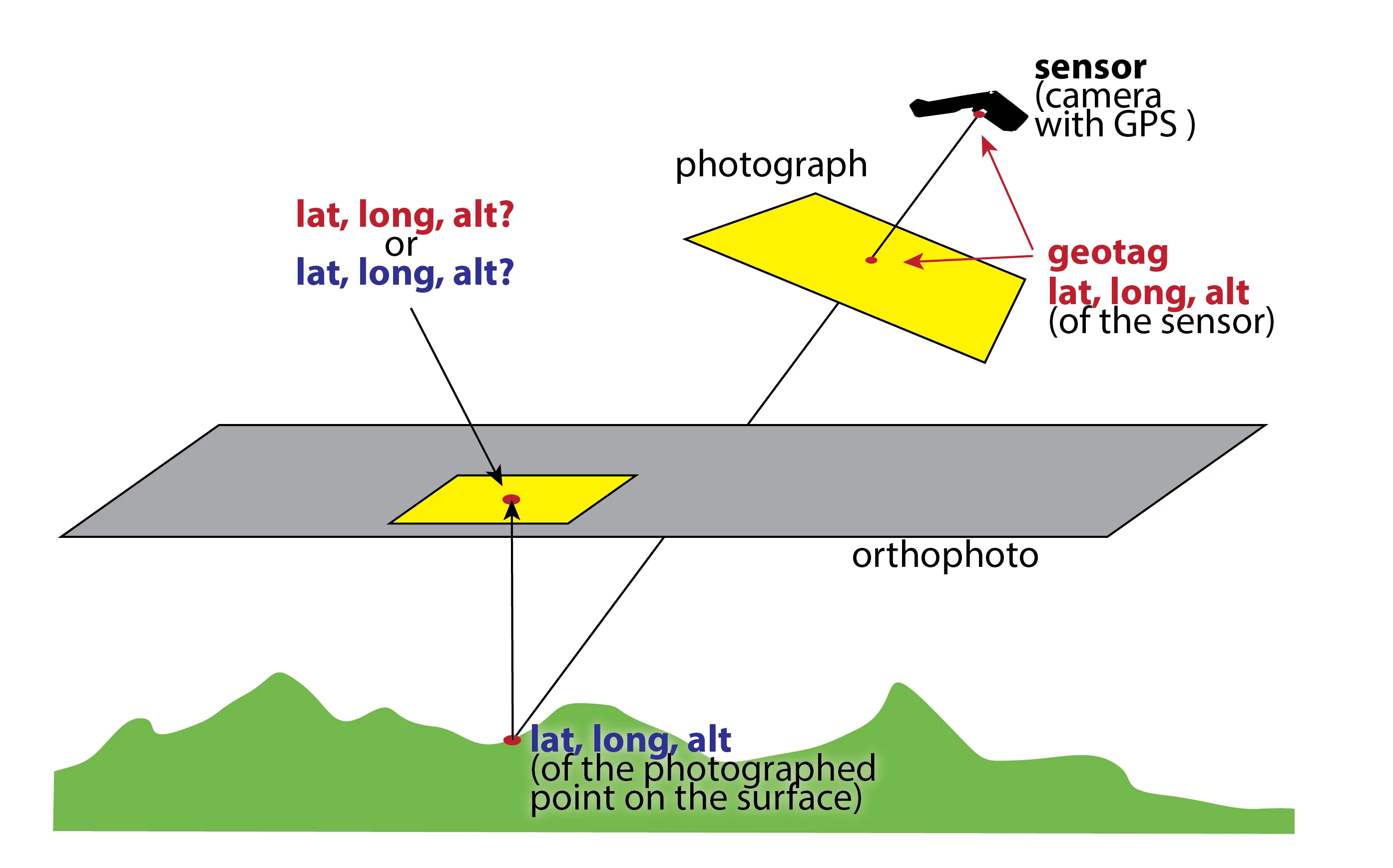
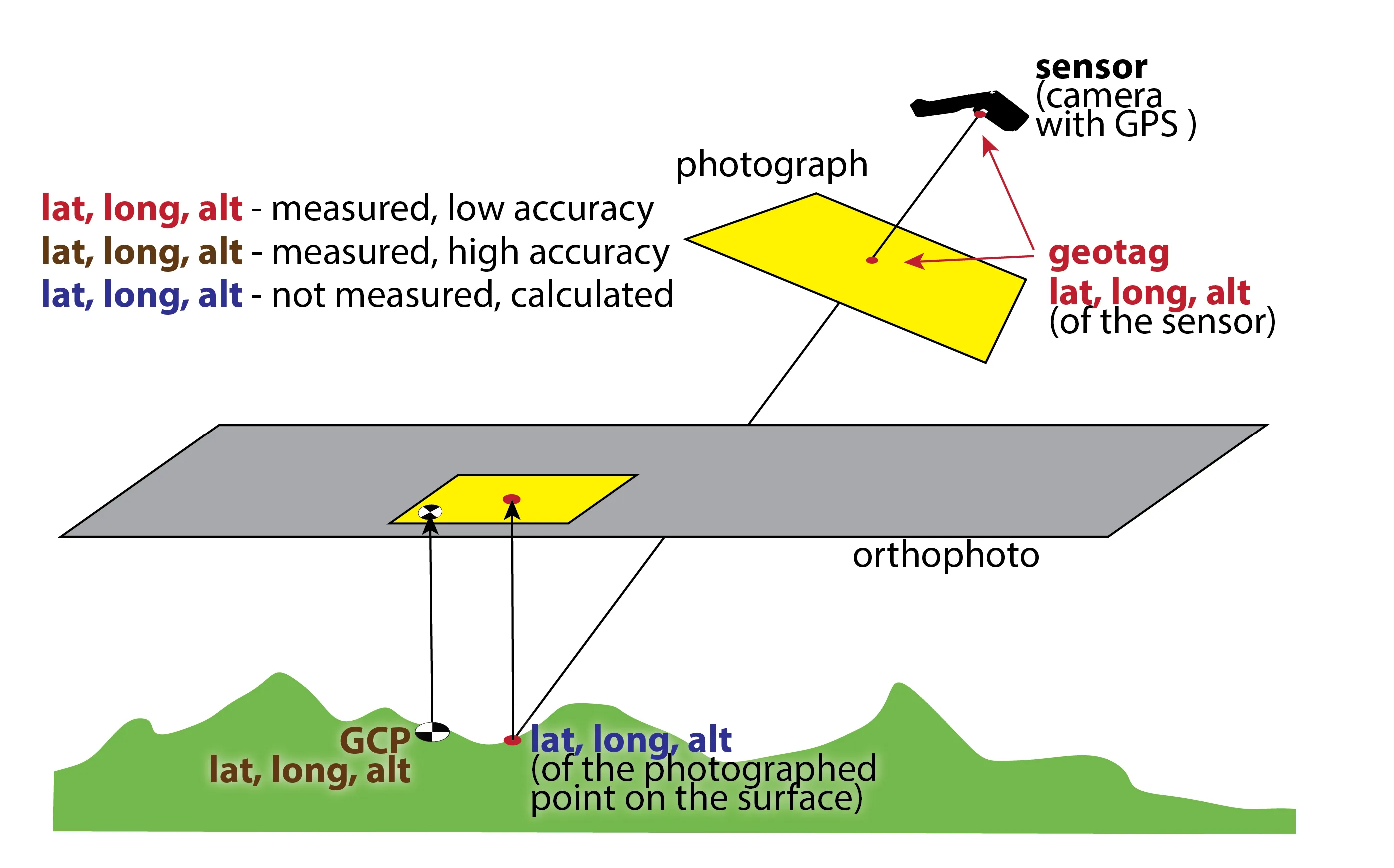
Whose coordinates are these?
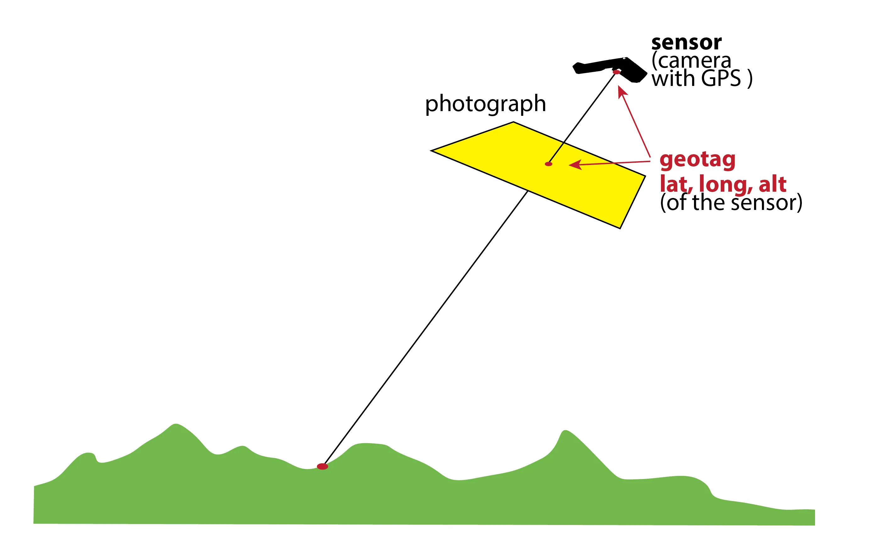
A camera with GPS above terrain; the geotag gives the latitude, longitude, and altitude of the sensor

The same diagram asking whether the orthophoto pixel takes the coordinates of the sensor or of the photographed ground point

The diagram with three coordinate types: geotag measured at low accuracy, GCP measured at high accuracy, ground point calculated

Geotags: useful, but not survey control

  • Written into each image’s EXIF by the aircraft GNSS: latitude, longitude, altitude, often attitude
  • Give the bundle adjustment a starting point and a rough scale and orientation
  • Consumer GNSS is accurate to 1 to 3 m horizontally and worse vertically; altitude is often barometric and relative to the takeoff point

Rule of thumb: geotags get the model into the right neighborhood; centimeter accuracy comes from RTK/PPK or ground control

Ground control points

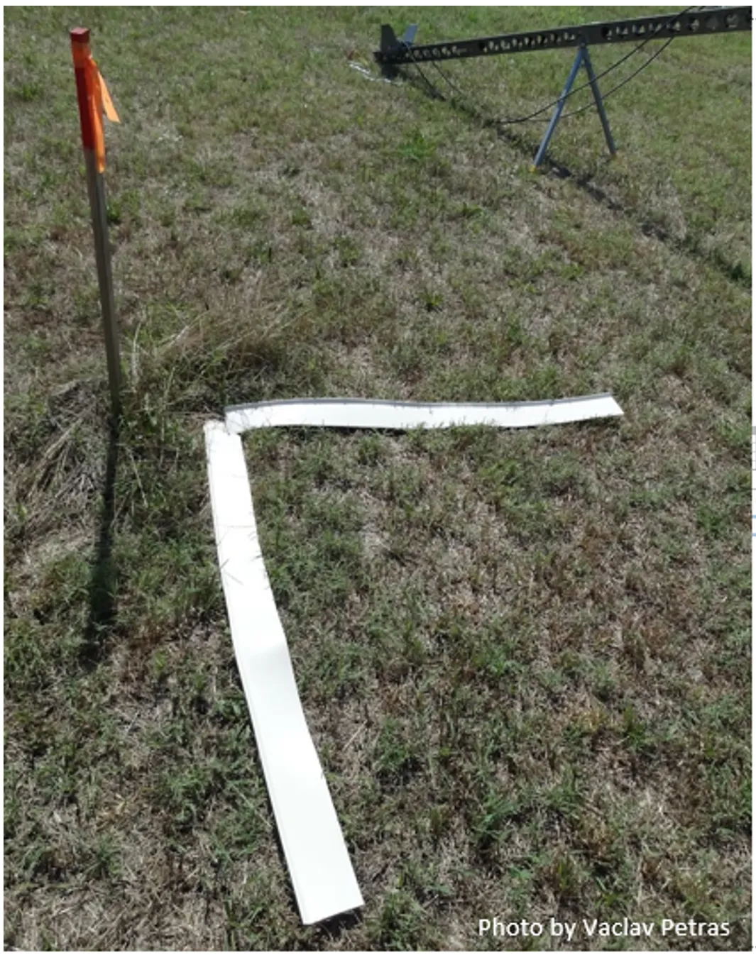
A white L-shaped ground control target and a survey flag on grass

A GCP target at Lake Wheeler. Photo by Vaclav Petras
  • A target on the ground whose center is surveyed to centimeter accuracy (RTK GNSS or total station)
  • Visible and unambiguous in the imagery: high contrast, larger than a few pixels at your GSD
  • Marked in several photos during processing; the software then adjusts the block to fit
  • Distributed across the whole area and the full range of elevation, including the edges
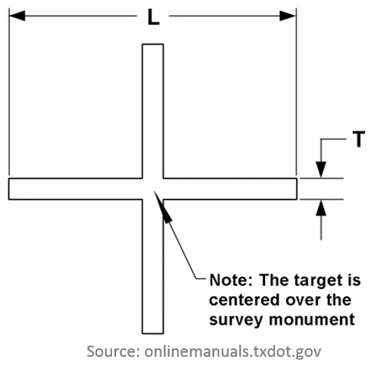
Sketch of a cross-shaped survey target centered over a survey monument

Control versus checkpoints

Ground control points (GCPs): used in the adjustment to constrain the solution

Checkpoints: surveyed the same way but withheld from the adjustment, used only to measure error

  • At least 3 GCPs to define the coordinate system; 5 or more spread across the site in practice
  • Report accuracy as RMSE on independent checkpoints, never on the GCPs themselves
  • If checkpoint error is much larger than GCP error, the model is overfitting the control

Direct georeferencing: RTK and PPK

Method Camera position accuracy Ground control needed Typical use
Standard GNSS geotags 1 to 3 m Yes, for any survey-grade product Consumer drones
RTK (real-time corrections) 1 to 3 cm Few; still use checkpoints Survey platforms with a base station or network
PPK (post-processed corrections) 1 to 3 cm Few; still use checkpoints Same, more tolerant of radio dropouts
GCPs only n/a 5 or more, well distributed Any platform, extra field time

Even with RTK/PPK: place a few checkpoints, and at least one GCP to fix any vertical offset, since camera accuracy is not the same as product accuracy

Common pitfalls

Symptom Cause Fix
Few tie points, images fail to align Low texture (water, sand, uniform crops, snow) or repetitive patterns Fly lower, add obliques, fly when shadows add texture
Smeared or duplicated features Rolling shutter, motion blur, wind Faster shutter, slower flight, global shutter camera
Flat site reconstructs as a dome or bowl Weak geometry and self-calibration error GCPs across the site, obliques, two flying heights
Surfaces under trees are wrong The model is a DSM: it sees the canopy, not the ground Compare to a DTM only after ground classification
Patchy colors, visible seams Changing light or exposure during the flight Manual exposure, fly in even light, avoid long flights across weather changes

Quick activity

In teams of three, sketch a plan for mapping a site of your choice:

  1. What do you want to measure, and to what accuracy?
  2. What GSD does that imply? (Just the target; the formula comes in Topic 3)
  3. Nadir only, or nadir plus oblique? What overlap? Test your overlap in the demo: how many photos does the plan need, and do all the points turn green?
  4. How many GCPs and checkpoints, and where?
  5. Which products do you need: orthophoto, DSM, DTM, point cloud, mesh?

Key terms

Parallax: the shift of a feature between photos taken from different positions; the source of all depth information in SfM

Tie point: a feature detected and matched across two or more photos

Bundle adjustment: the joint least-squares solution for camera poses, camera model, and 3D points that minimizes reprojection error

Interior and exterior orientation: the camera model (focal length, principal point, distortion) and each photo’s position and attitude

GCP and checkpoint: surveyed targets used to constrain the solution, and surveyed targets withheld to measure its error

GSD: the ground size of one pixel; set by focal length, sensor, and flying height (formula in Topic 3)

Wrap-up

Assignment 2A: 3D reconstruction from multiple photos, photograph an object, build a model, and report what helped and what hurt the reconstruction

Next lecture: UAS imagery processing, the full pipeline from images to orthophoto and DSM in Agisoft Metashape

References

This deck adapts and extends the original course slides (Jeziorska and Mitasova 2016). For the mathematics of dense matching see Furukawa and Hernández (2015); for a longer treatment of SfM for the geosciences see OpenTopography (2021).

Furukawa, Yasutaka, and Carlos Hernández. 2015. “Multi-View Stereo: A Tutorial.” Foundations and Trends in Computer Graphics and Vision 9 (1-2): 1–148. https://doi.org/10.1561/0600000052.
Jeziorska, Justyna, and Helena Mitasova. 2016. Photogrammetry and Structure from Motion Concepts. GIS 584 UAS Mapping and Analytics course slides, Center for Geospatial Analytics, NC State University.
OpenTopography. 2021. Introduction to Structure from Motion Photogrammetry. Geological Society of America 2021 short course, lectures and demos. https://opentopography.org/workshops/GSA2021.

Image credits

  • Camera geometry: Natural Resources Canada
  • Perspective versus orthographic projection: Wikipedia
  • Relative and absolute orientation: Q. Abdullah, Penn State GEOG 892
  • SfM diagram: theia-sfm.org
  • Analog orthophoto instruments: USGS
  • GCP target sketch: TxDOT survey manual
  • 1906 San Francisco kite photographs: G. Lawrence, Library of Congress
  • Tie-point and geotag sequences, overlap diagram, GCP photo: NC State Center for Geospatial Analytics