Ground Control, Checkpoints, and Accuracy

Center for Geospatial Analytics at North Carolina State University

Corey White

Objectives

  • Relate flight GSD to the horizontal and vertical accuracy a UAS survey can reach
  • Design ground control and checkpoint schemes
  • Choose between GCP-based and RTK/PPK georeferencing
  • Read an Agisoft or WebODM processing report
  • Determine the level of detection (LoD)

The report number is not the accuracy

A worked example from the ASPRS standard (American Society for Photogrammetry and Remote Sensing 2024):

  • The DSM fits the checkpoints with RMSEV1 = 1 cm
  • The checkpoints themselves were surveyed with an RTK rover: RMSEV2 = 2 cm
  • You may claim the quadrature sum: \(\text{RMSE}_V = \sqrt{1^2 + 2^2} = 2.24\) cm
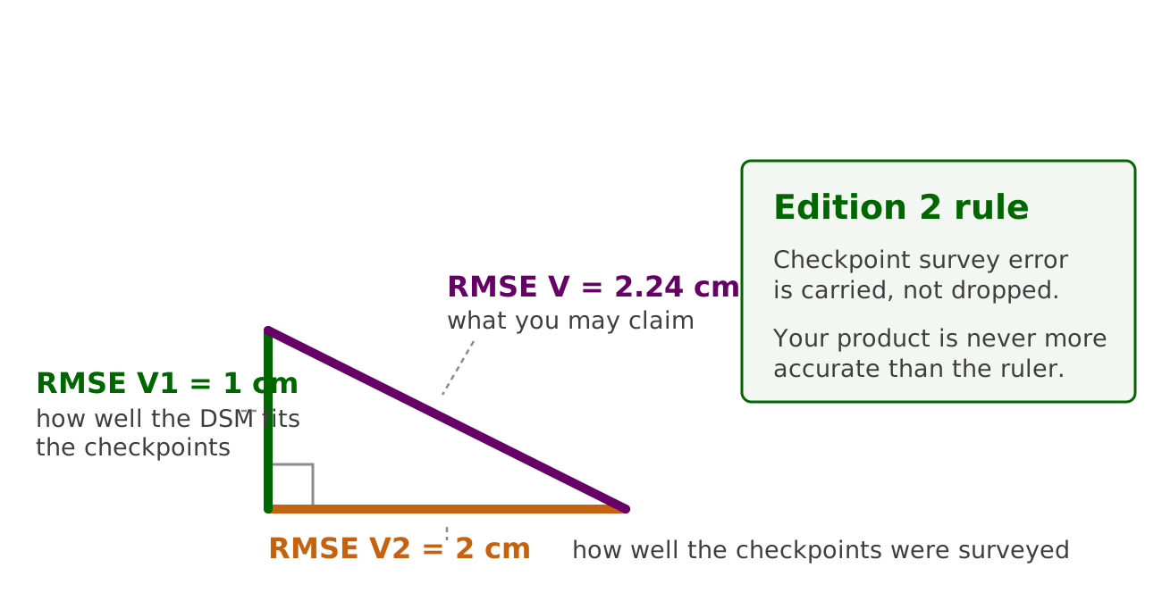
A right triangle with a 1 cm vertical leg for the DSM fit, a 2 cm horizontal leg for the checkpoint survey, and a 2.24 cm hypotenuse for the accuracy that may be claimed

What GSD buys you

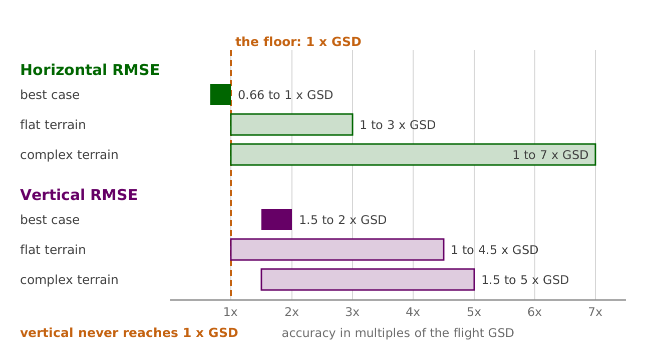
GSD sets a floor, not the accuracy

Bar chart of horizontal and vertical RMSE in multiples of GSD: horizontal best case 0.66 to 1x, flat terrain 1 to 3x, complex terrain 1 to 7x; vertical best case 1.5 to 2x, flat terrain 1 to 4.5x, complex terrain 1.5 to 5x
  • Envelopes from Jiménez-Jiménez et al. (2021); best case from Sanz-Ablanedo et al. (2018)
  • Vertical error runs about 2.5 x the horizontal error (Sanz-Ablanedo et al. 2018)
  • With uncorrected navigation-grade georeferencing, errors reach meters and pixel size stops mattering

Planning with GSD

flowchart LR
    A["What you must<br>measure"] --> B["The accuracy<br>that requires"]
    B --> C["GSD:<br>0.5 to 1.0 x that"]
    C --> D["Flying height<br>(Topic 3A)"]

  • ASPRS recommends source imagery GSD of 0.5 to 1.0 x the target horizontal accuracy class: a 5 cm class wants 2.5 to 5 cm GSD (American Society for Photogrammetry and Remote Sensing 2024)
  • Read backwards: expect RMSEH of 1 to 2 x GSD from a well-run project
  • The standard calls this a planning heuristic and says it may not be used to report accuracy

Ground control

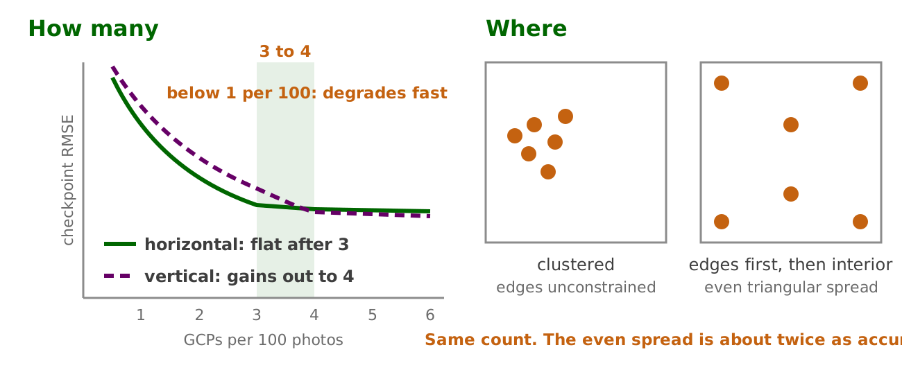
How many GCPs, and where

Left panel: checkpoint RMSE against GCPs per 100 photos, horizontal flattening after 3 and vertical still gaining out to 4. Right panel: a clustered GCP layout beside an even layout with points on the edges and interior
  • About 3 to 4 GCPs per 100 photos; below 1 per 100 accuracy degrades fast (Sanz-Ablanedo et al. 2018)
  • Edge coverage first, then an even interior; points past that improve error structure rather than RMSE (Dai et al. 2023)

Control at Lake Wheeler
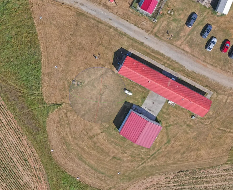
Orthomosaic of the Lake Wheeler barn and surrounding fields from the September 2026 flight, with checkerboard ground control targets visible on the ground around the buildings

Our own flight. Targets ring the site: a few become control, the rest stay checkpoints.

Control is not validation
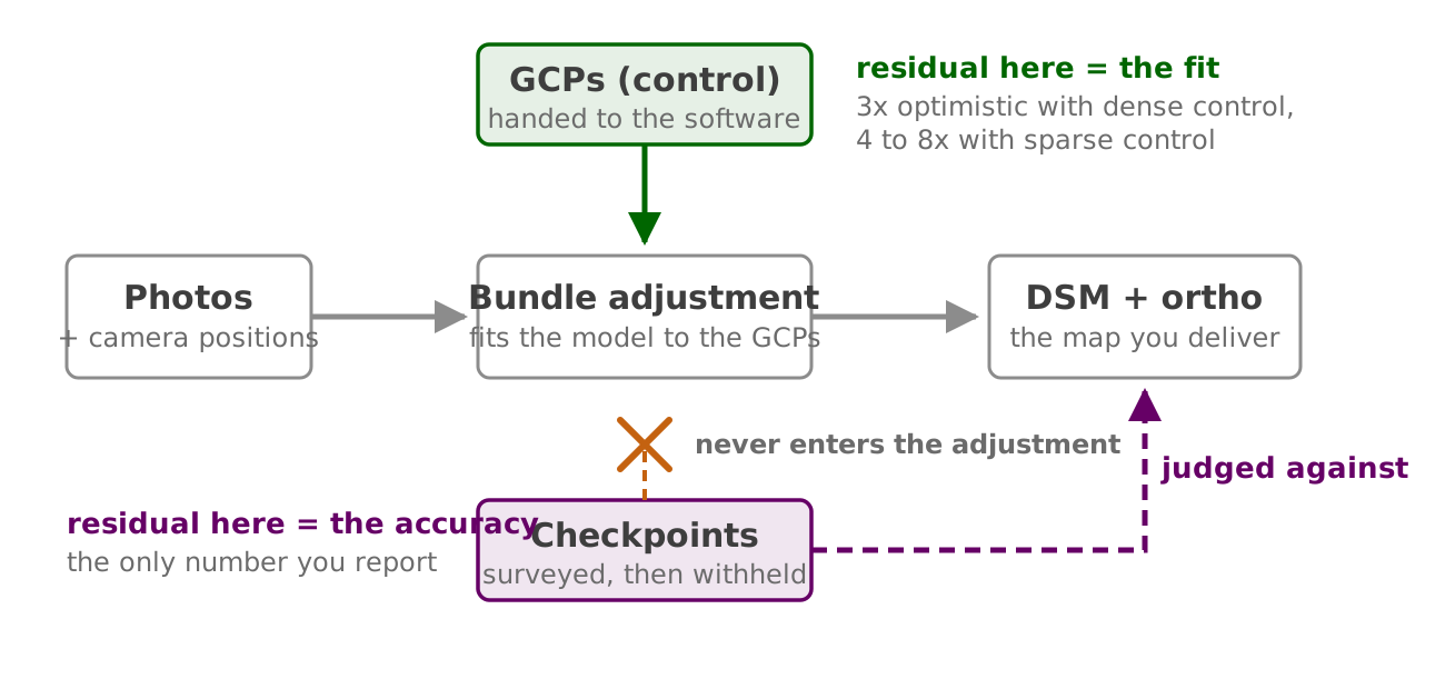
Flow diagram: GCPs feed the bundle adjustment which produces the DSM and orthomosaic, while checkpoints bypass the adjustment entirely and are used to judge the product

RTK, PPK, and what they still need

Direct georeferencing today

Evidence Result
ASPRS Addendum V (American Society for Photogrammetry and Remote Sensing 2024) PPK reaches 1 to 2 cm horizontal, 2 to 4 cm vertical “when used properly”; RTK typically 5 to 10 cm
RTK aircraft, zero GCPs, purpose-built flight (Stott et al. 2020) Vertical RMSE 6.6 cm over 2 km of river; adding 5 GCPs did not improve it
PPK versus GCP workflows (Zhang et al. 2019) PPK matched GCP-workflow accuracy (MAE about 2 cm, RMSE about 3 cm); some missions carried a vertical bias that one GCP removed, improving vertical accuracy 20 to 30 percent
Repeat surveys (Nota et al. 2022) Co-alignment of epochs gives sub-2 cm relative accuracy; ground control in at least one epoch still anchors absolute Z

Where the standard disagrees

Working defaults: RTK or PPK for georeferencing, 1 or 2 GCPs to control the vertical datum, every other surveyed point withheld as a checkpoint

  • ASPRS keeps GCPs “highly recommended” and gives them priority over airborne positions in the adjustment: camera centers have fewer epochs and weaker geoid handling than survey-grade ground occupations (American Society for Photogrammetry and Remote Sensing 2024)
  • The journal results assume strong flight geometry; the standard is written for contracts and courts

The base coordinate governs everything
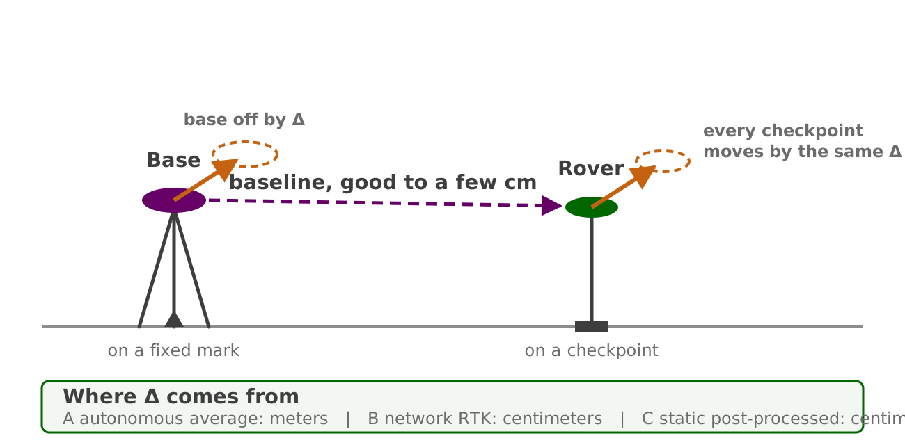
A base station on a fixed mark and a rover on a checkpoint joined by a baseline vector; an offset in the base coordinate shifts the rover position by the same amount
  • Base within 0.5 mm: an Emlid Reach RS2 base gave DEM vertical RMSE of 1.94 cm versus 1.89 cm for a Trimble Alloy with a choke-ring antenna (Famiglietti et al. 2021), at roughly a tenth of the price
  • Antenna beats receiver: a low-cost dual-frequency board matched geodetic instruments in network RTK only with a geodetic-grade antenna; with a patch antenna it needed open sky (Janos and Kuras 2021)

Systematic error

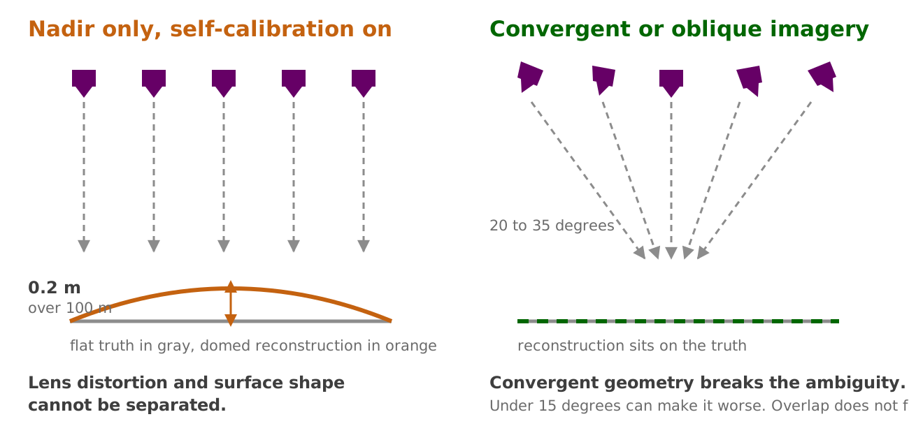
Doming

Left: parallel nadir views over a flat surface produce a domed reconstruction about 0.2 m high over 100 m. Right: convergent views tilted 20 to 35 degrees produce a reconstruction that sits on the true surface
  • Camera orientations off parallel by only 2 degrees produce a dome of about 0.2 m over 100 m (James and Robson 2014)
  • Fixes in order of power: a known camera model with self-calibration off; oblique imagery (a convergent orbit reached under 2 mm in simulation); two flying heights; well-distributed control
  • Best camera angles in the tested 0 to 35 degree range were 20 to 35 degrees, worth nearly 50 percent better accuracy in high relief (Nesbit and Hugenholtz 2019)
  • A gently tilted camera (under 15 degrees) can make things worse on consumer wide-angle cameras with onboard lens correction (James et al. 2020)

Why systematic error matters more
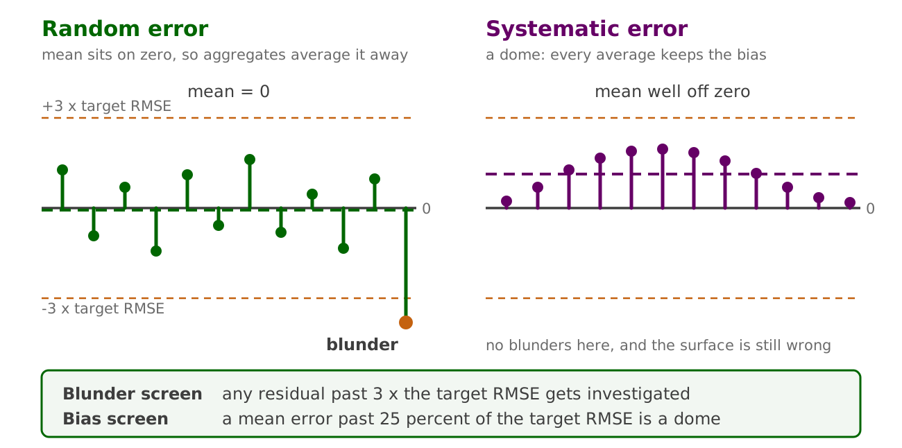
Two panels of checkpoint residuals about a zero line: random error with a mean on zero and one blunder past the three sigma screen, and systematic error shaped like a dome with the mean well off zero

Reading the reports

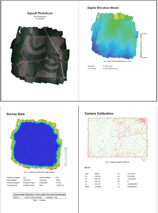
A processing report, page by page

Four pages of an Agisoft processing report: the survey overview with the reconstructed model, the digital elevation model, the survey data page with the camera location and overlap figure, and the camera calibration page with the residual plot

Survey overview, DEM, survey data with the overlap figure, camera calibration with residuals.

Where you declare your ruler
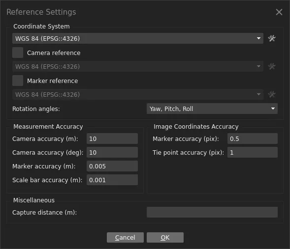
Metashape Reference Settings dialog showing camera accuracy of 10 m, marker accuracy of 0.005 m, and image coordinate marker accuracy of 0.5 pixels

Marker accuracy is RMSEV2. The software weights the adjustment with it, then reports a fit that still does not include it.

The same facts in two reports

Quantity Agisoft Metashape report WebODM quality report
GSD Survey Data: ground resolution Overview: average GSD
Coverage and photos Survey Data: coverage area, aligned images Overview: area, reconstructed images
Overlap Camera locations and image overlap figure Survey Data overlap heatmap
Camera model Calibrated values with uncertainties and residual plot Camera parameters, per-band
Camera position error Camera Locations table: X, Y, Z error GPS/geolocation details, 3D errors
Control fit Ground Control Points table: control RMSE GCP errors section (when GCPs used)
Checkpoint error Check Points rows in the same table Absent unless checkpoints were declared

What neither report tells you

  • Whether the checkpoints were independent; the software trusts your labeling
  • The survey accuracy of the control and checkpoints, so neither can do the quadrature for you
  • Whether the error is spatially structured: a mean near zero can hide a dome that cancels
  • Anything about the parts of the site with no checkpoints

Report vocabulary (American Society for Photogrammetry and Remote Sensing 2024): report RMSEH and RMSEV (RMSE3D if asked); Edition 2 drops the old 95 percent confidence reporting; 30 checkpoints is the minimum for a statistical claim, and Section 7.16.1 gives the wording for when you have fewer

What can you measure

The level of detection

\[\text{LoD} = 1.96 \sqrt{\sigma_{z1}^2 + \sigma_{z2}^2} \approx 2.8\,\sigma_z\]
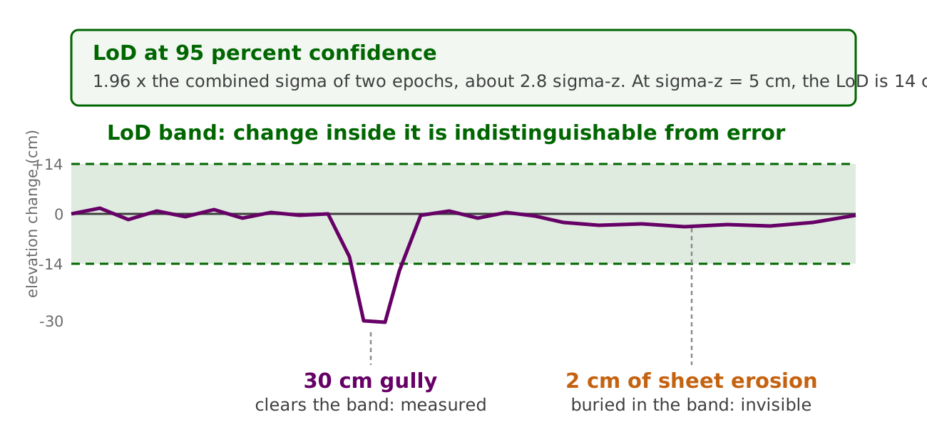
An elevation difference profile with a shaded plus or minus 14 cm level of detection band; a 30 cm gully punches below the band while 2 cm of sheet erosion stays inside it
  • Thresholding is for gross change only; it biases net change, where random errors already cancel (Anderson 2019)
  • Spatially variable LoD can exclude from a quarter to more than half of observed volumetric change (Wheaton et al. 2010)

Trees or erosion

Question Binding constraint Verdict at 3 cm GSD, 5 cm sigma-z
Count the trees Detection in the orthomosaic Easy; accuracy barely matters
Measure canopy height Canopy and ground surfaces, not GSD: flying height 80 to 120 m showed no significant effect on tree height RMSE (1.8 to 3.2 m) (Grybas and Congalton 2022) Expect meters of error regardless of pixel size
Detect a 30 cm rill or gully LoD about 14 cm Yes, cleanly
Quantify 2 cm sheet erosion LoD, dominated by systematic error No; needs sub-2 cm sigma-z, near-ground flights, and bias control

Key terms

Checkpoint: surveyed, withheld, judges the map; also called check point, validation point, independent test point

Direct georeferencing: camera positions from RTK or PPK doing the work of control; also called GNSS-aided or GCP-free

Level of detection (LoD): the smallest elevation change distinguishable from error at a stated confidence

Doming: broad systematic DEM deformation from the self-calibration ambiguity; also called bowling when inverted

RMSEH, RMSEV, RMSE3D: Edition 2’s reporting quantities, replacing RMSEx/RMSEy/RMSEz and the 95 percent statistics

Quadrature: accuracies add as the square root of summed squares; the product carries the checkpoint survey error

Wrap-up

Assignment 3B: Validate the Lake Wheeler flight: establish the base coordinate three ways, evaluate the flight’s orthomosaic and DSM against the checkpoints you collected, and rule on what the flight can measure

Midterm 11/4: the control versus checkpoint distinction, the quadrature rule, and the LoD arithmetic are all fair game

References

American Society for Photogrammetry and Remote Sensing. 2024. ASPRS Positional Accuracy Standards for Digital Geospatial Data, Edition 2, Version 2. American Society for Photogrammetry; Remote Sensing. https://publicdocuments.asprs.org/PositionalAccuracyStd-Ed2-V2.
Anderson, Scott W. 2019. “Uncertainty in Quantitative Analyses of Topographic Change: Error Propagation and the Role of Thresholding.” Earth Surface Processes and Landforms 44 (5): 1015–33. https://doi.org/10.1002/esp.4551.
Dai, Wen, Ruibo Qiu, Bo Wang, et al. 2023. “Enhancing UAV-SfM Photogrammetry for Terrain Modeling from the Perspective of Spatial Structure of Errors.” Remote Sensing 15 (17): 4305. https://doi.org/10.3390/rs15174305.
Famiglietti, Nicola Angelo, Gianpaolo Cecere, Carmine Grasso, Antonino Memmolo, and Annamaria Vicari. 2021. “A Test on the Potential of a Low Cost Unmanned Aerial Vehicle RTK/PPK Solution for Precision Positioning.” Sensors 21 (11): 3882. https://doi.org/10.3390/s21113882.
Grybas, Heather, and Russell G. Congalton. 2022. “Evaluating the Impacts of Flying Height and Forward Overlap on Tree Height Estimates Using Unmanned Aerial Systems.” Forests 13 (9): 1462. https://doi.org/10.3390/f13091462.
James, Mike R., Gilles Antoniazza, Stuart Robson, and Stuart N. Lane. 2020. “Mitigating Systematic Error in Topographic Models for Geomorphic Change Detection: Accuracy, Precision and Considerations Beyond Off-Nadir Imagery.” Earth Surface Processes and Landforms 45 (10): 2251–71. https://doi.org/10.1002/esp.4878.
James, Mike R., and Stuart Robson. 2014. “Mitigating Systematic Error in Topographic Models Derived from UAV and Ground-Based Image Networks.” Earth Surface Processes and Landforms 39 (10): 1413–20. https://doi.org/10.1002/esp.3609.
Janos, Daniel, and Przemysław Kuras. 2021. “Evaluation of Low-Cost GNSS Receiver Under Demanding Conditions in RTK Network Mode.” Sensors 21 (16): 5552. https://doi.org/10.3390/s21165552.
Jiménez-Jiménez, Sergio Iván, Waldo Ojeda-Bustamante, Mariana de Jesús Marcial-Pablo, and Juan Enciso. 2021. “Digital Terrain Models Generated with Low-Cost UAV Photogrammetry: Methodology and Accuracy.” ISPRS International Journal of Geo-Information 10 (5): 285. https://doi.org/10.3390/ijgi10050285.
Nesbit, Paul Ryan, and Christopher H. Hugenholtz. 2019. “Enhancing UAV-SfM 3D Model Accuracy in High-Relief Landscapes by Incorporating Oblique Images.” Remote Sensing 11 (3): 239. https://doi.org/10.3390/rs11030239.
Nota, E. W., W. Nijland, and T. de Haas. 2022. “Improving UAV-SfM Time-Series Accuracy by Co-Alignment and Contributions of Ground Control or RTK Positioning.” International Journal of Applied Earth Observation and Geoinformation 109: 102772. https://doi.org/10.1016/j.jag.2022.102772.
Sanz-Ablanedo, Enoc, Jim H. Chandler, José Ramón Rodríguez-Pérez, and Celestino Ordóñez. 2018. “Accuracy of Unmanned Aerial Vehicle (UAV) and SfM Photogrammetry Survey as a Function of the Number and Location of Ground Control Points Used.” Remote Sensing 10 (10): 1606. https://doi.org/10.3390/rs10101606.
Stott, Eilidh, Richard D. Williams, and Trevor B. Hoey. 2020. “Ground Control Point Distribution for Accurate Kilometre-Scale Topographic Mapping Using an RTK-GNSS Unmanned Aerial Vehicle and SfM Photogrammetry.” Drones 4 (3): 55. https://doi.org/10.3390/drones4030055.
Wheaton, Joseph M., James Brasington, Stephen E. Darby, and David A. Sear. 2010. “Accounting for Uncertainty in DEMs from Repeat Topographic Surveys: Improved Sediment Budgets.” Earth Surface Processes and Landforms 35 (2): 136–56. https://doi.org/10.1002/esp.1886.
Zhang, He, Emilien Aldana-Jague, François Clapuyt, Florian Wilken, Veerle Vanacker, and Kristof Van Oost. 2019. “Evaluating the Potential of Post-Processing Kinematic (PPK) Georeferencing for UAV-Based Structure-from-Motion (SfM) Photogrammetry and Surface Change Detection.” Earth Surface Dynamics 7 (3): 807–27. https://doi.org/10.5194/esurf-7-807-2019.