Classification methods for UAS data
Center for Geospatial Analytics at North Carolina State University
Outline
- Pixel, Object, Image Classification
- Supervised vs Unsupervised learning
- Segmentation
- Feature Extraction
- Model Selection and Validation
- Real-time UAS analysis
What is image classification?
- Labling images with sematic lables
Car, house, lake, tree, forest, etc..
Image classification applications
- Land cover/land use classifcation
- Flood detection
- Species Identifcation
- Surveillance
- Object Tracking
UAS Data Characteristics
- High spatial resolution (1–10 cm)
- Limited spectral bands (RGB or multispectral)
- High within-class variability
- Shadows, BRDF effects, and illumination differences
Pixel-based classification
Each pixel is given a semantic label
Object-based classification
The image is segmented into objects (groups of pixels) and the objects are classified
Semantic Scene classification
The entire image is classified into a semantic scene
Machine Learning Methods
- Supervised Learning
- Unsupervised Learning
- Deep Learning
Supervised Learning
Labeled features are used to train ML model
May require significant amount of training data.
Subject to the nonstationarity nature of spatial-temporal data
Random Forest, Gradient Boot, SVM
Unsupervised Learning
Data is classified through statistical modeling.
No training data is required
Classes are not defined and require interpretation
k-means, ISODATA
Deep Learning
- Artificial Neural Network (ANN)
- Convolutional Neural Network (CNN)
- Deep Neural Networks (UNET, )
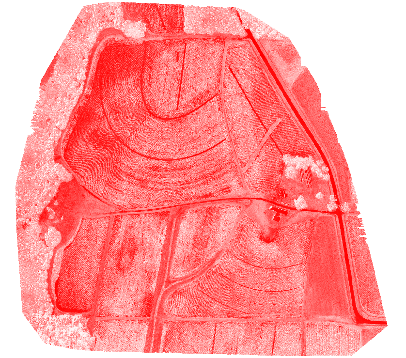
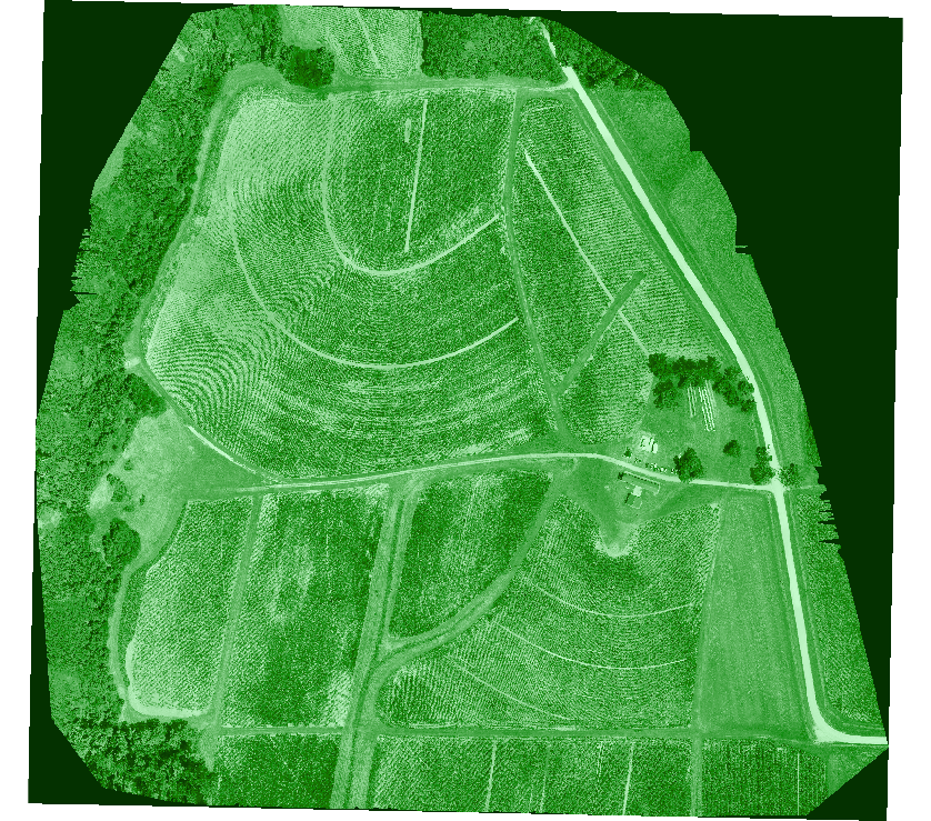
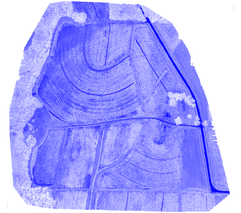
Spectral Properties
- Every surface has a unique spectral reflectance curve
- UAS sensors capture reflected light in discrete bands:
- Red, Green, Blue (visible)
- NIR (if multispectral)
- Thermal
- etc..
- Used to derive spectral indices for classification
Common Spectral Indices
| NDVI |
(NIR - Red) / (NIR + Red) |
Vegetation health |
| VARI |
(G - R) / (G + R - B) |
Green vegetation from RGB |
| NDWI |
(G - NIR) / (G + NIR) |
Water detection |
| NDBI |
(SWIR - NIR) / (SWIR + NIR) |
Built-up detection |
Feature Engineering
- Normalized Indices
- Low and High Pass Filters
- Low Pass - Smoothing Kernal
- High Pass - Edge Detection
- Textural features
- Grey level co-occurrence matrix (GLCM)
- Angular Second Moment
- Contrast
- Correlation
- Geometric Characteristics
- Principal component analysis (PCA)
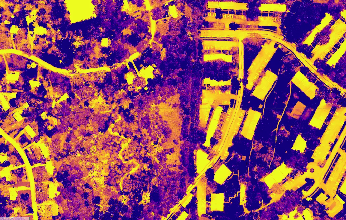
![VARI]() \[
VARI = \frac{(Green - Red)}{(Green + Red - Blue)}
\]
\[
VARI = \frac{(Green - Red)}{(Green + Red - Blue)}
\]
Sampling Methods
- Random Sample
- Sample the entire spatial extent \(n\) number of locations
- Cluster Sampling
- Sample by different clusters
- Stratified Random Sample
- Sample by different classes (e.g. Developed, Undeveloped)
Training a model
- Break data into training and testing dataset 80/20
- Avoid overfitting data
- May require a large volume of data
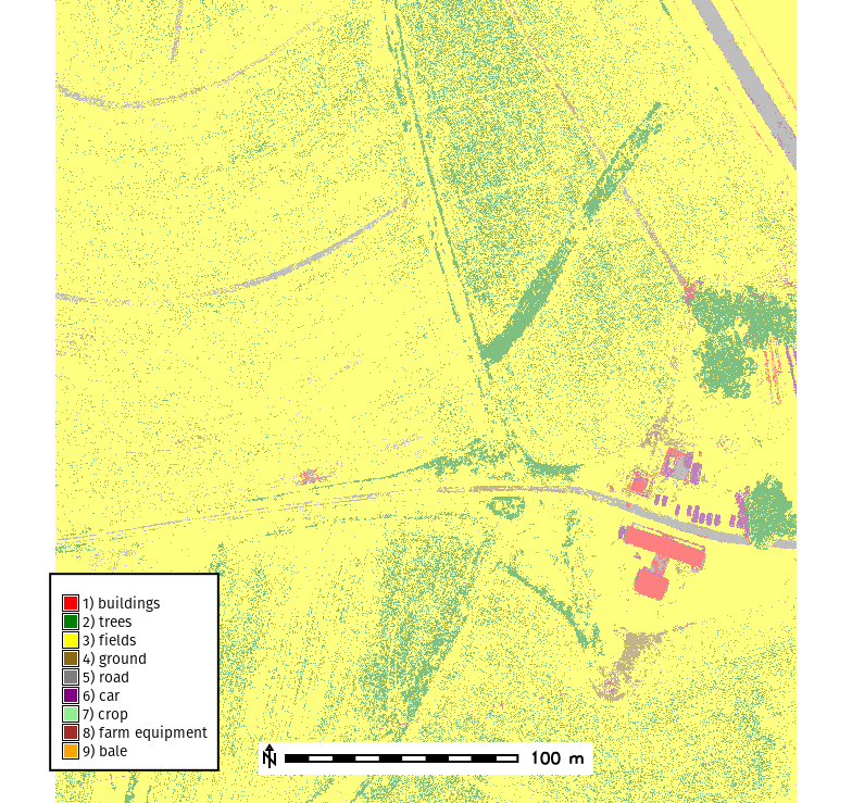
Classification Results
![]()
Model Validation
Confusion Matrix
| Forest |
50 |
2 |
3 |
0 |
90.9 |
| Water |
1 |
45 |
0 |
4 |
88.2 |
| Urban |
2 |
1 |
40 |
7 |
80.0 |
| Agriculture |
0 |
3 |
5 |
42 |
85.7 |
| Producer’s Accuracy (%) |
94.3 |
86.5 |
83.3 |
79.2 |
|
- \(Overall\ Accuarcy = \frac{Correctly\ classified\ samples}{Total\ samples}\)
- Kappa coefficient (Cohen’s Kappa): inter-rater agreement
Challenges
- Handling multiple spatial scales
- Nonstationarity
- Processing/Training
 \[
VARI = \frac{(Green - Red)}{(Green + Red - Blue)}
\]
\[
VARI = \frac{(Green - Red)}{(Green + Red - Blue)}
\]