Introduction
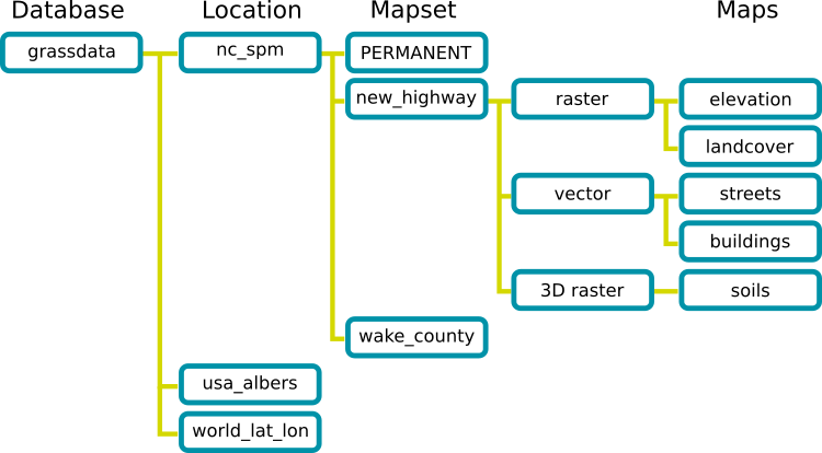
Start and GRASS data structure
For this introduction we create new mapset intro to keep data organized.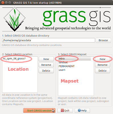
Display
Add raster map
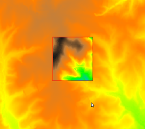
Let's add raster map called elev_lid792_1m to the Layer Manager so that it is displayed in the Map Display. You can either use the add raster icon in the toolbar or you can use main menu File → Map display → Add raster. Then select raster map from the selection.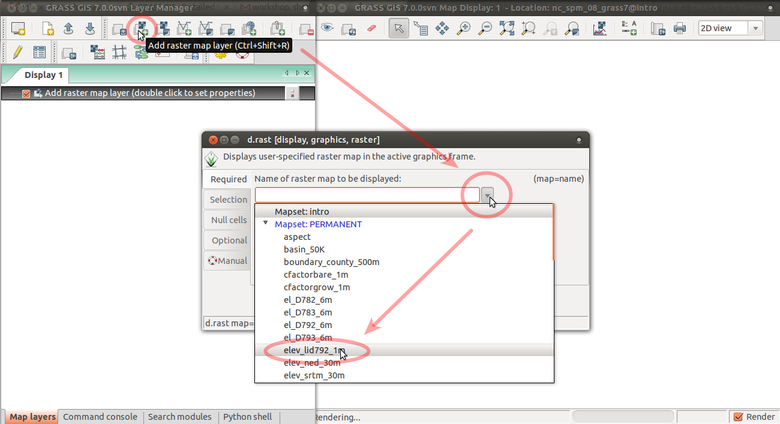
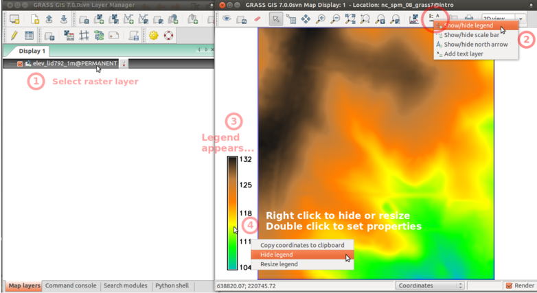
Display legend
GRASS modules
GRASS functionality is available through modules (tools). Modules respect following naming conventions:
| group | prefix | examples |
|---|---|---|
| general | g.* | g.list, g.remove, g.copy |
| raster | r.* | r.univar, r.neighbors, r.contour |
| vector | v.* | v.info, v.generalize, v.db.select |
| imagery | i.* | i.segment, i.cluster, i.colors.enhance |
| 3D raster | r3.* | r3.info, r3.to.rast, r3.colors |
| temporal | t.* | t.list, t.rast.aggregate, t.vect.univar |
| ... | ... | ... |
Finding and running a module
Tp find a module for your analysis, type the term into the search box in the Search modules tab, keep pressing Enter until you find your module.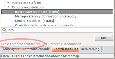
Running a module as a command
If you already know the name of the module, you can just use it in the command line. The GUI offers a Command console tab with command line specifically build for running GRASS GIS modules. If you type module name there, you will get suggestions for automatic completion of the name. After pressing Enter, you will get GUI dialog for the module.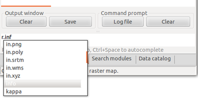
Module parameters
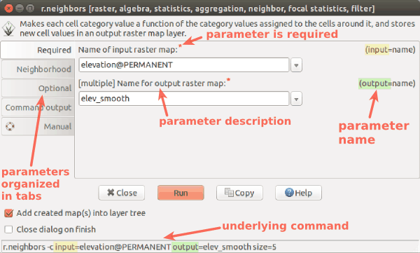
r.neighbors -c input=elevation output=elev_smooth size=5
Region settings
Before we use a module to compute a new raster map, we must set properly computational region. All raster computations will be performed in the specified extent and with the given resolution. The numeric values of computational region can be checked using:
g.region -p
north:      220750
south:      220000
west:       638300
east:       639000
nsres:      1
ewres:      1
rows:       750
cols:       700
cells:      525000
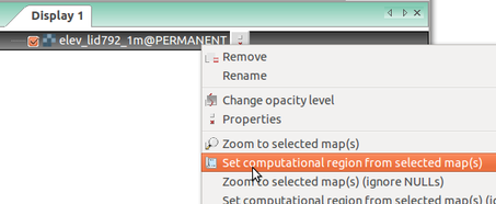
Set the computational extent and resolution of the mapset to match map
elev_lid792_1m.
We can set it to match a raster map like this:
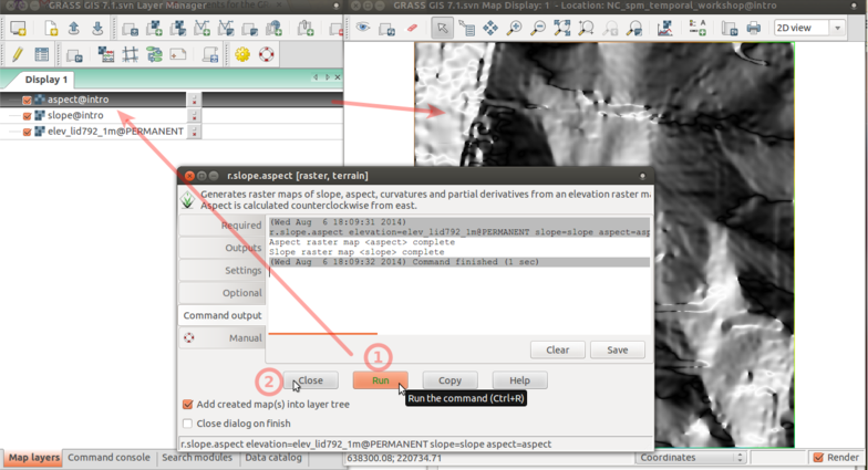
Running modules
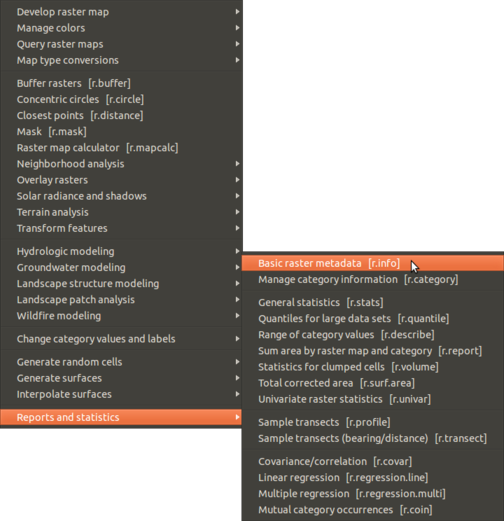
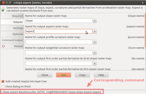
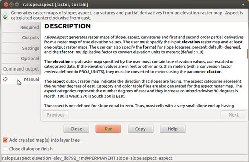
Find the module for computing slope and aspect in menu or the module tree under Raster → Terrain analysis → Slope and aspect or simply run r.slope.aspect.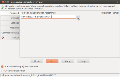
Learn more
- Getting started with GRASS GIS GUI video
- GRASS GIS GUI (graphical user interface manual)
- Understanding module GUI dialogs
- Similar introduction as a web page and as PDF slides
- Browse GRASS GIS modules: by topic, by keyword and by individual modules