UAS and lidar data: comparison, fusion, and analysis
GIS/MEA 584:
Mapping and Analysis Using UAS
Helena Mitasova, Anna Petrasova, Justyna Jeziorska
Center for Geospatial Analytics,
North Carolina State University
Outline
- Motivation for combining lidar and UAS SfM data
- Analysis of lidar and UAS SfM DSMs differences
- Patching and smooth fusion of UAS and lidar DSM
- Overland flow simulation on fused DEM
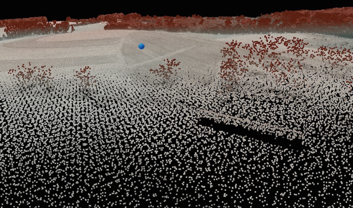
Point clouds from lidar
- measured variable is time of return for each pulse
- georeferencing is based on the position (measured by GPS) and exterior orientation (measured by inertial navigation system INS) of the platform
- (x,y,z) is derived from time, GPS positioning and INS parameters
Point clouds from SfM
- measured variable is reflected energy captured as imagery
- georeferencing can be done entirely from GCPs
- (x, y, z) is derived from overlapping images and GCPs
- alternatively: GPS and INS for position and orientation of images and camera parameters
Comparison of point cloud properties
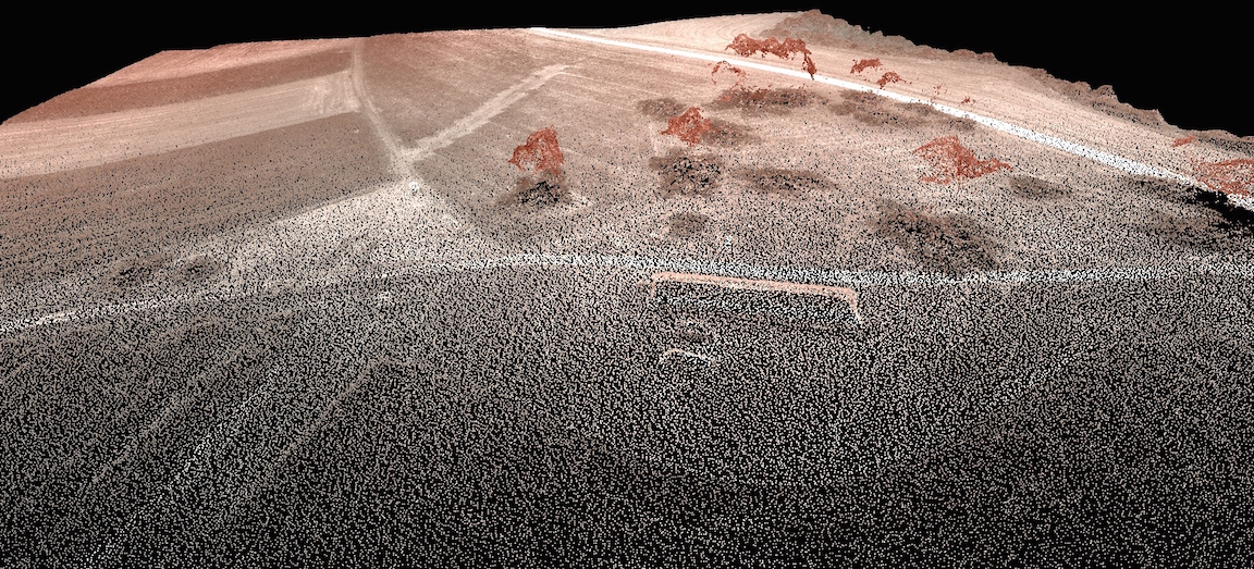
- Airborne Lidar:
- passes through vegetation,multiple return,
- shifts between swaths, cordurroy effect
- regional coverage
- high cost
-
UAS SfM:
- very high point density,
- limited capability to map under vegetation
- influenced by cast shadows,
- low cost, but limited area
Different distribution of errors and distortions: Lidar and SfM provide independent set of measurements.
Motivation for lidar and UAS SfM fusion
- low cost DEM updates in rapidly changing landscapes - e.g. construction sites
- replacing vegetated areas in UAS SfM by bare ground
- watershed analysis when only part of the watershed was mapped by UAS
- improve accuracy and level of detail over stable features (buildings, bridges)
- add your suggestion
Fusion techniques
- merge the point clouds, decimate or bin at high resolution, interpolate: computationally demanding
- interpolate DEMs, randomly sample, patch, and reinterpolate: loss of detail, time consuming
- interpolate DEMs and patch: sharp edges
- smooth fusion - requires DEMs at same resolution
Workflow
- evaluate the point clouds, select resolution
- interpolate lidar and UAS DEMs at the same resolution
- evaluate the differences between the lidar and UAS DEMs
- if applicable, identify errors and apply corrections
- apply smooth fusion
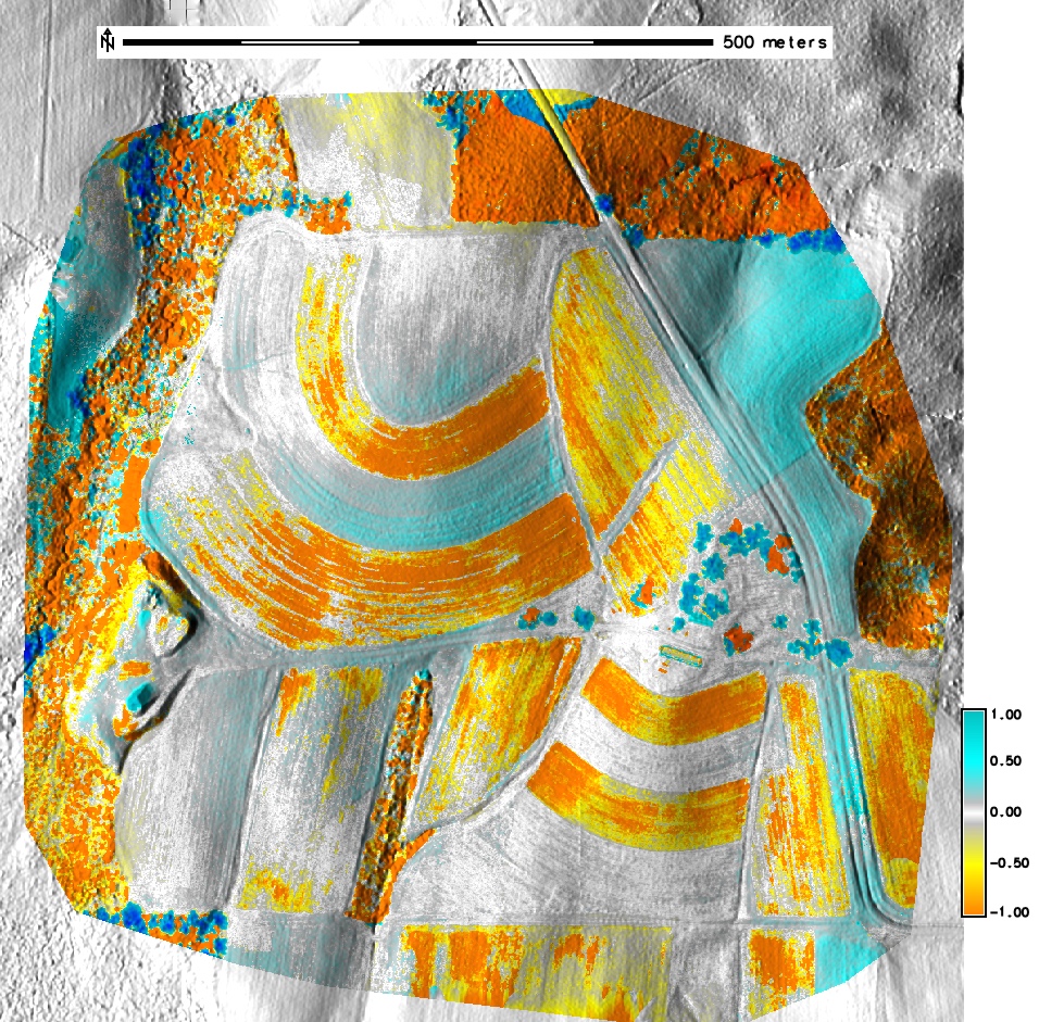
Identify distortions due to processing
- identify spatial pattern of distortions
- difference maps between Lidar DSM and UAS SfM DSMs: different distortions from AGISOFT and PIX4D
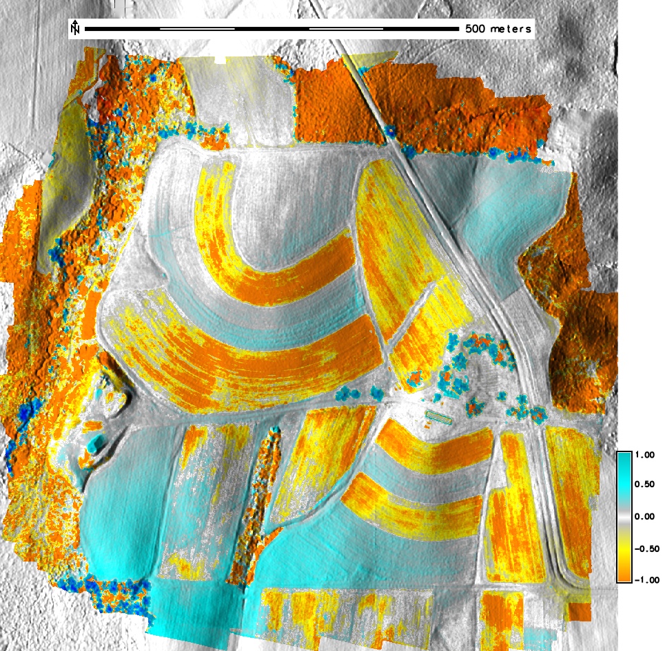
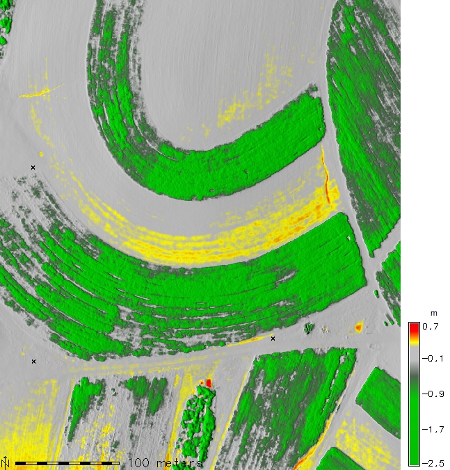
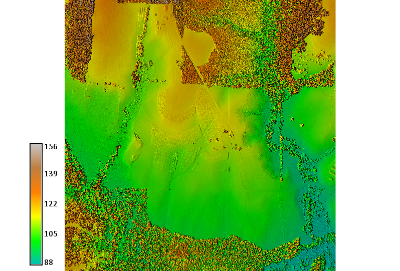
Identify changes in topography
- vegetation growth or removal
- change in elevation surface due to erosion processes
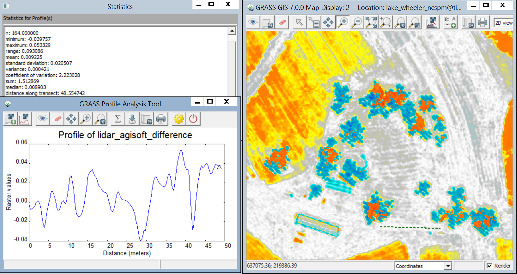
- UAS SfM - lidar difference maps with custom color
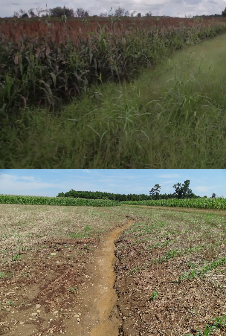
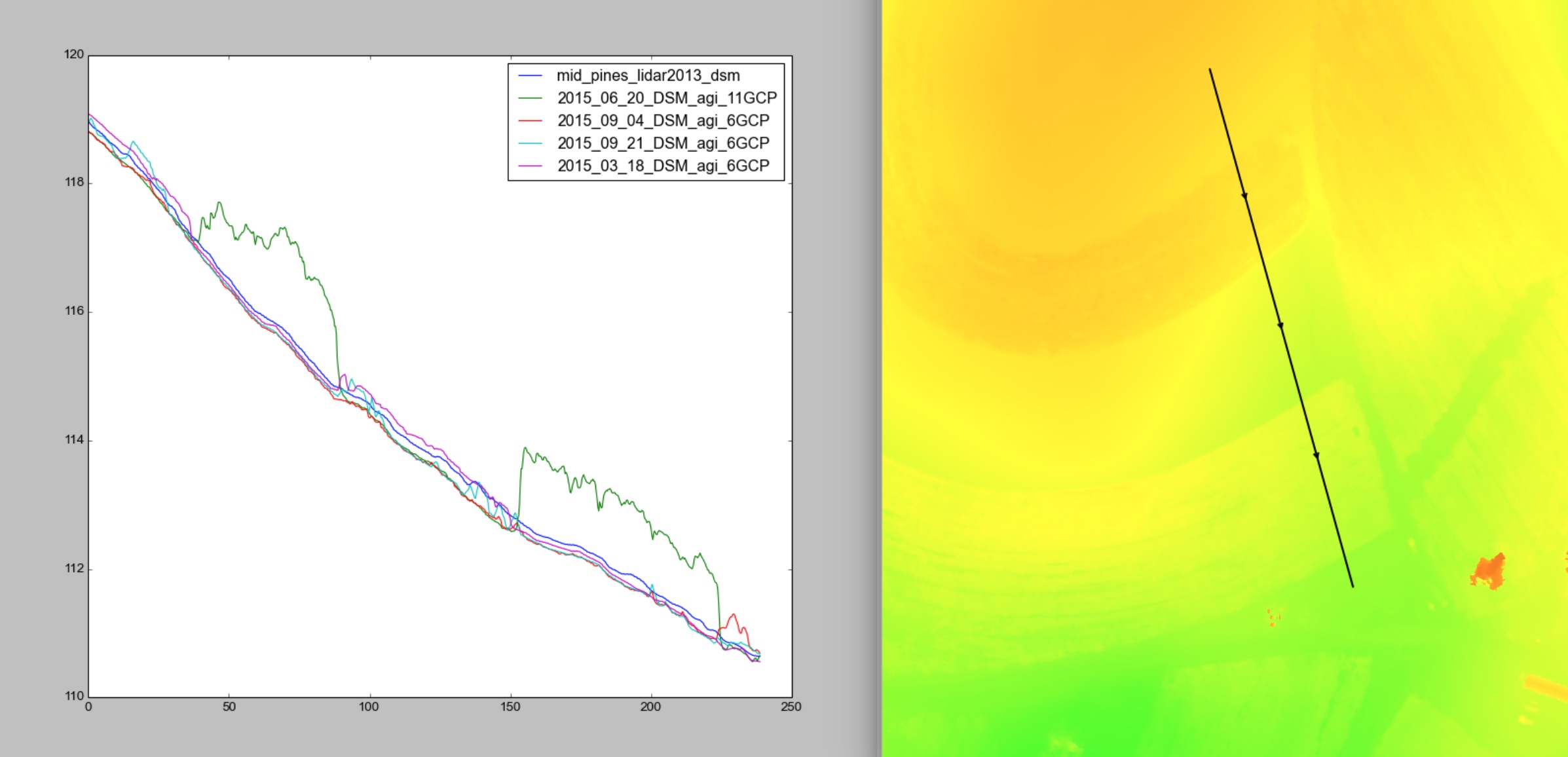
Comparing profiles: fields
- identify systematic errors (vertical shifts)
- differences due to vegetation growth, erosion/deposition
Comparing profiles: building
- high accuracy, lower level of detail in lidar data
- negligible systematic error
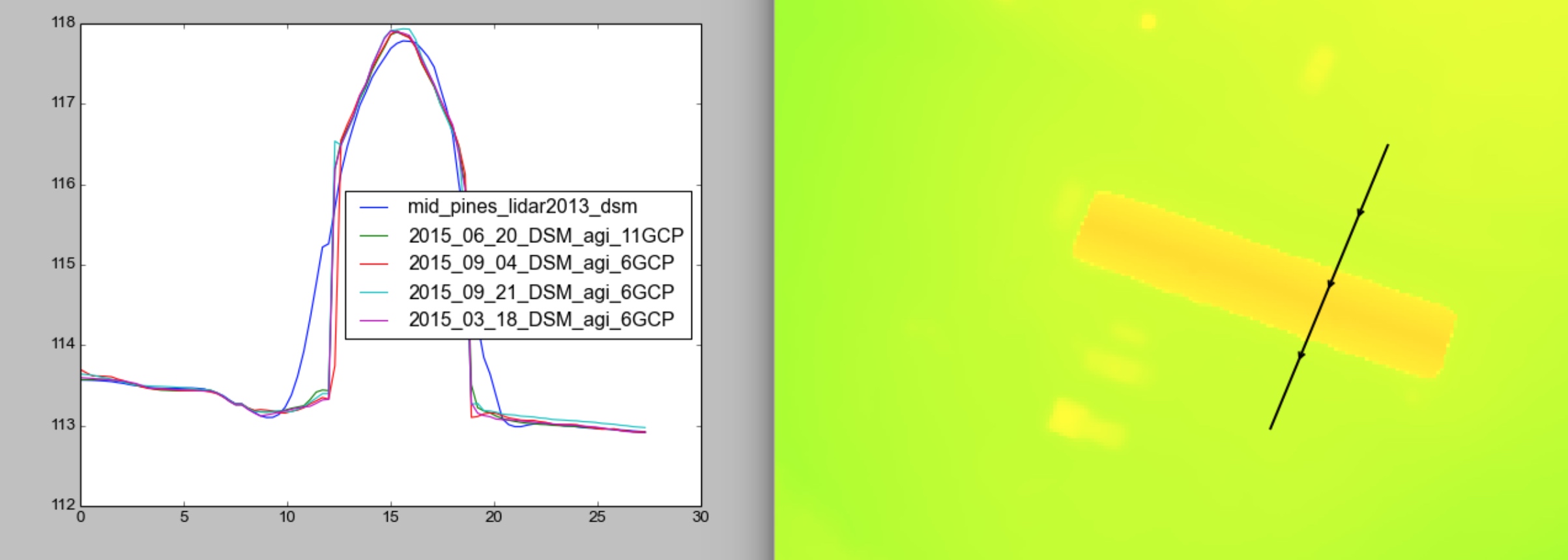
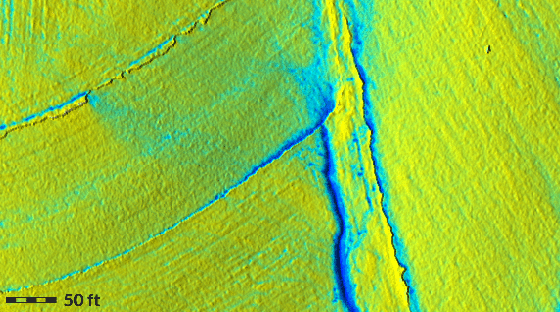
Comparing profiles: road
- relatively, easy to identify, stable feature
- high accuracy - differences between lidar and UAS SfM within 4cm
Correct for systematic error and distortions
- systematic error - if due to GPS shift, use median difference
- systematic error - if tilt, use regression function
- most challenging are complex UAS SfM distortions - they can be reduced using interpolated GCP differences or differencing with lidar
- importance of well distributed, accurate GCPs
Updating lidar DEM by patching
- replace the grid cells in the updated area by UAS DEM
- average over an overlap
- usually creates an edge - requires post-processing
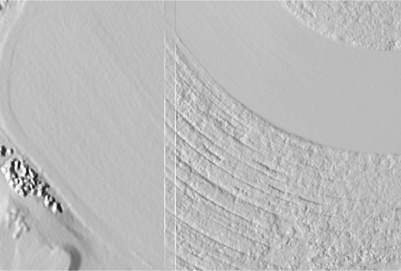
images by Brendan Harmon
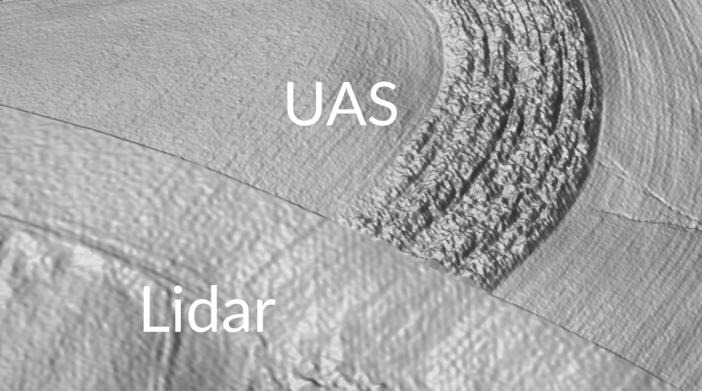
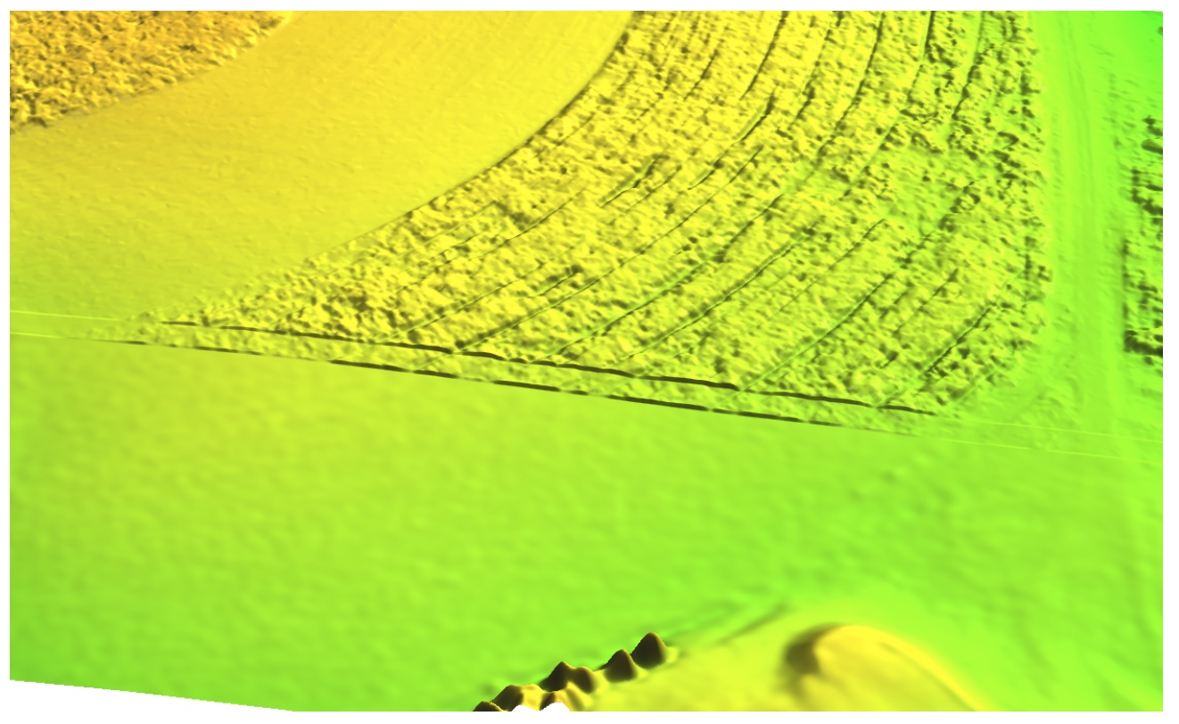
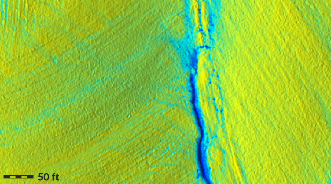
Updating lidar DEM by patching
edge between lidar and UAS SfM DEMs
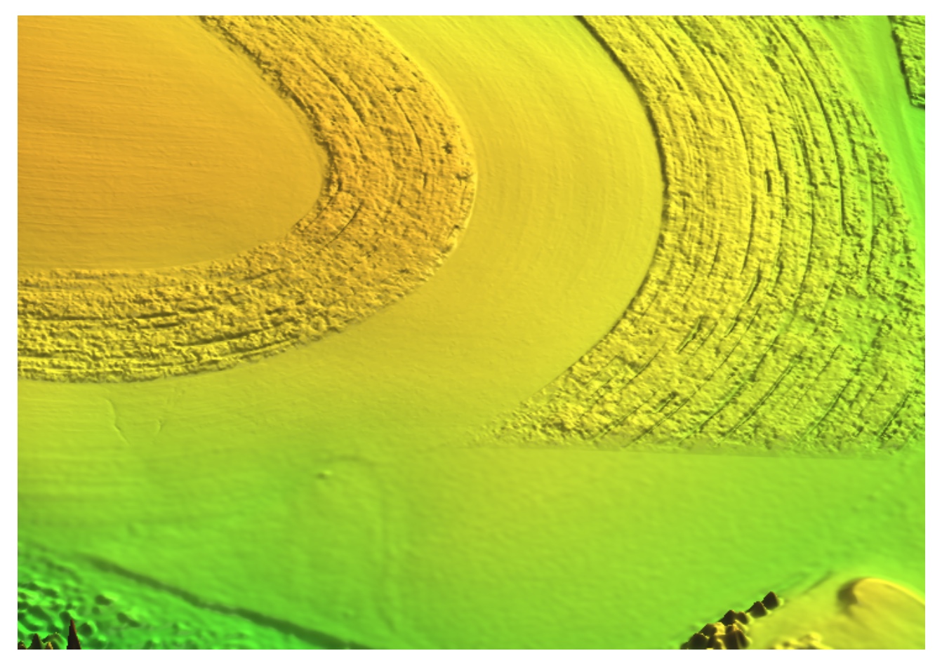
Smooth fusion
- derive overlap raster
- weighted smoothing based on the distance from the edge
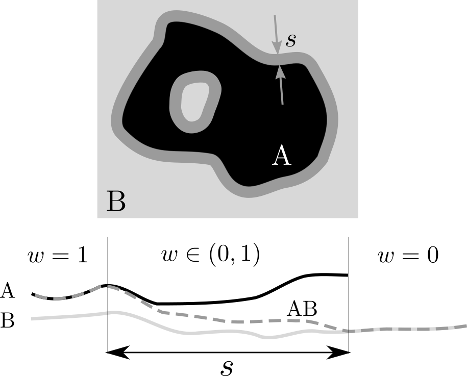
Fusion method
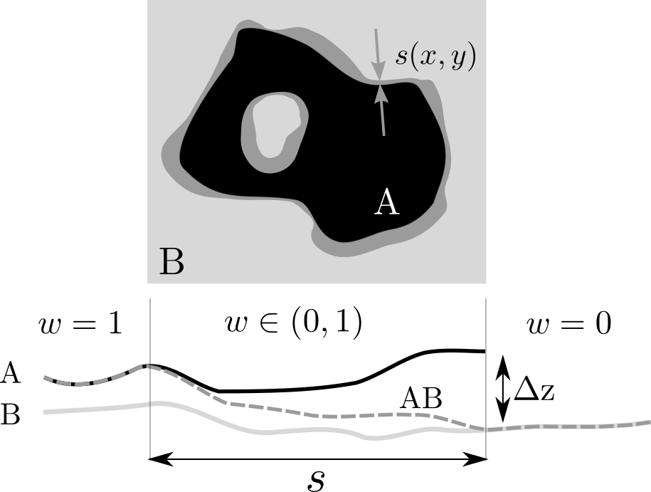
Linear combination of elevation surfaces $z_{A}$ and $z_{B}$ with weights given by overlap width $s$ and distance $d$ to the edge of $z_{A}$:
$$ z_{AB} = z_{A} w + z_{B}(1 - w), \\[10pt] w = f(s, d) = \begin{cases} \frac{d}{s} & 0 \leq d < s \\ 1 & d \geq s \end{cases} $$
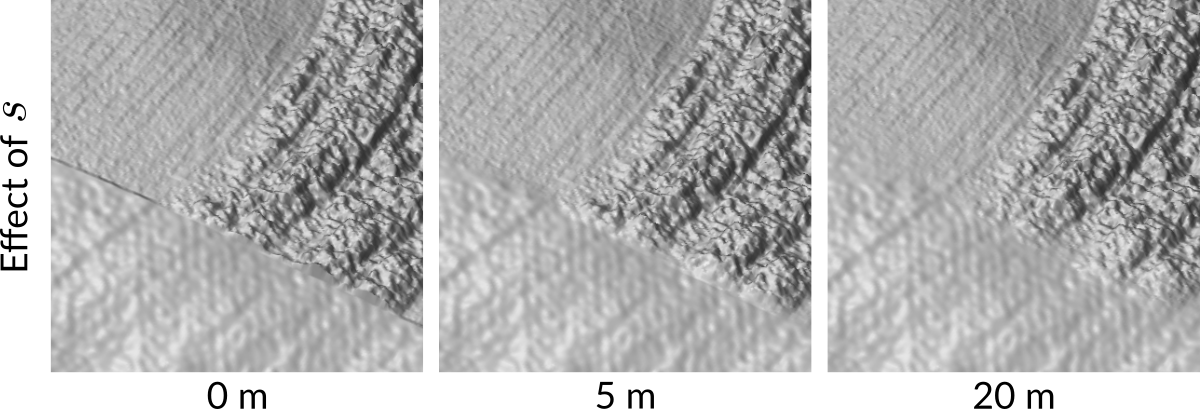
Influence of overlap width $s$
Fusion with spatially variable $s$
By taking into account spatially variable differences $\Delta z$ between DEMs $A$ and $B$ along the overlap:
- we get more gradual transition where differences are high
- we preserve subtle features of both DEMs where differences are small
Fusion with spatially variable $s$
Absolute elevation difference between lidar and UAS DEM controls the width of the transition overlap.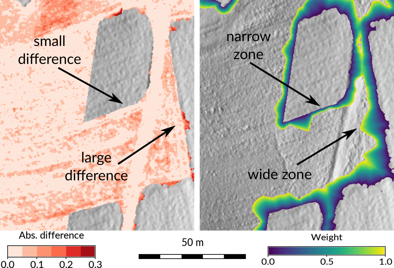
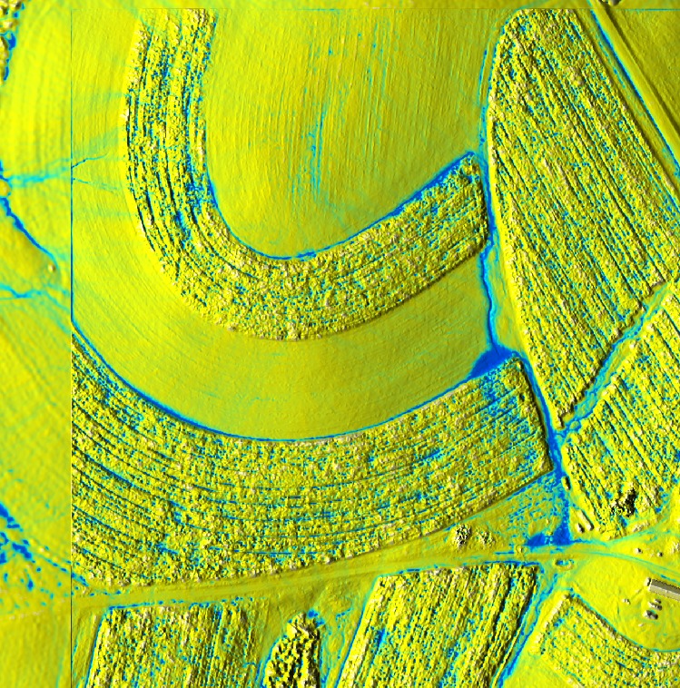
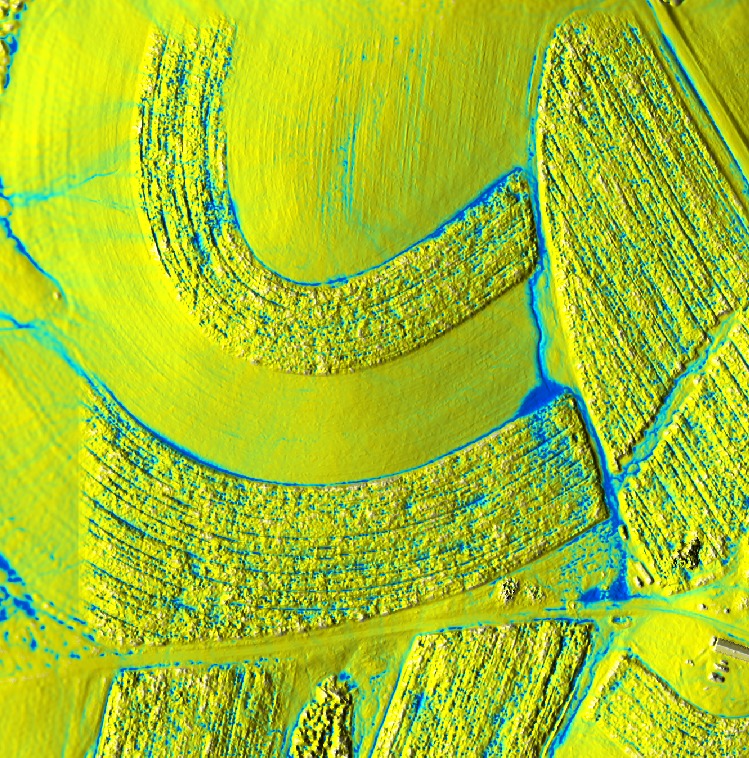
Lidar and UAS SfM patching and fusion
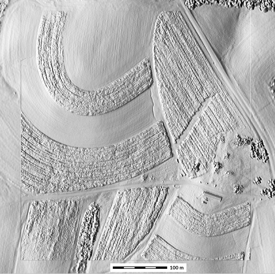
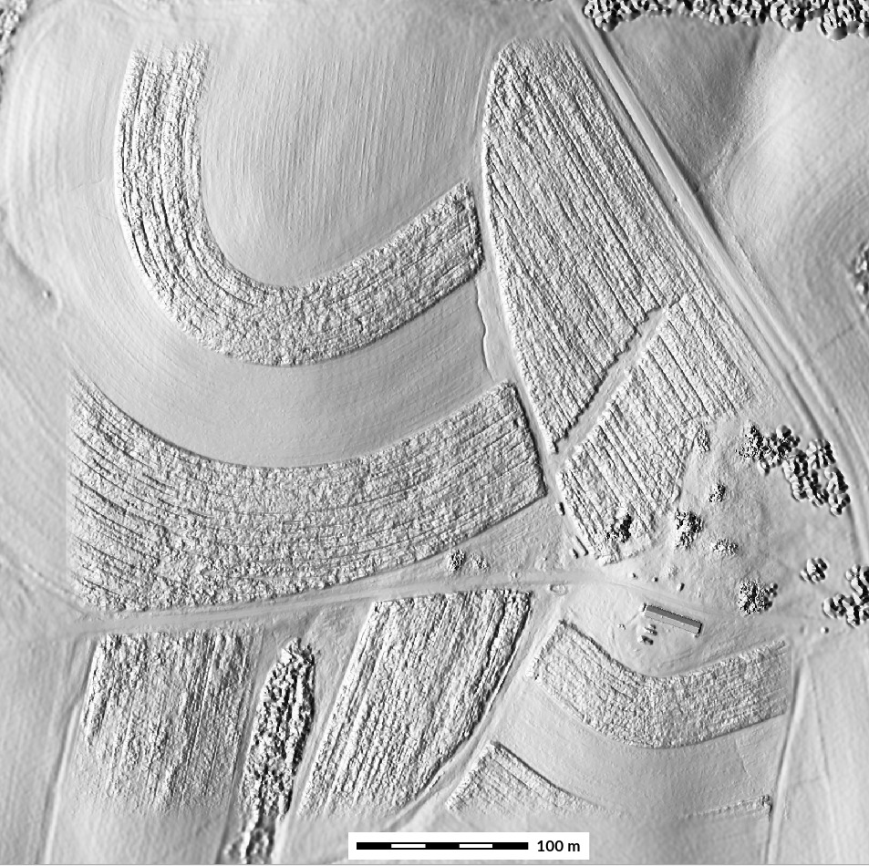
Simply patched vs. fused UAS and lidar DSMs with overlap width $s = 20\ m$
Fusing vegetated patch with bare ground
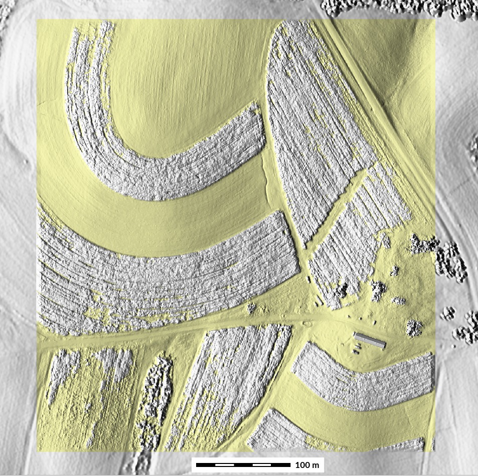
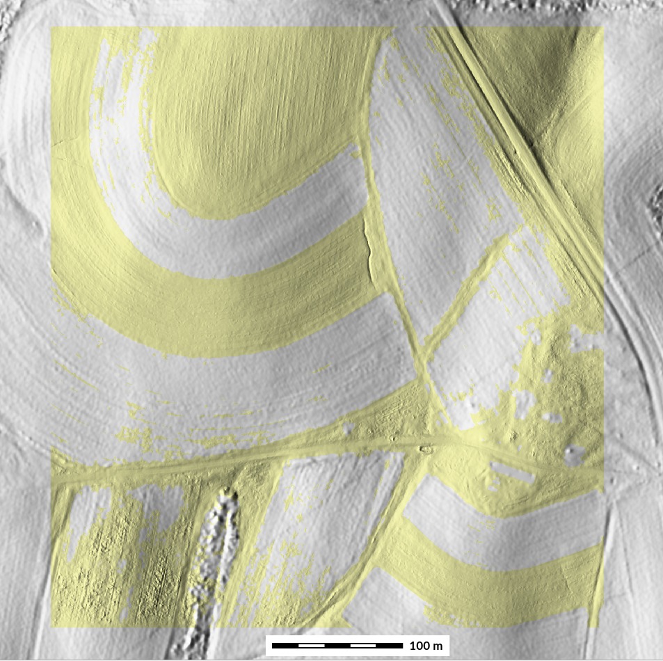
Vegetated areas in UAS DSM are replaced with lidar DEM. Yellow shows bare ground in UAS DSM.
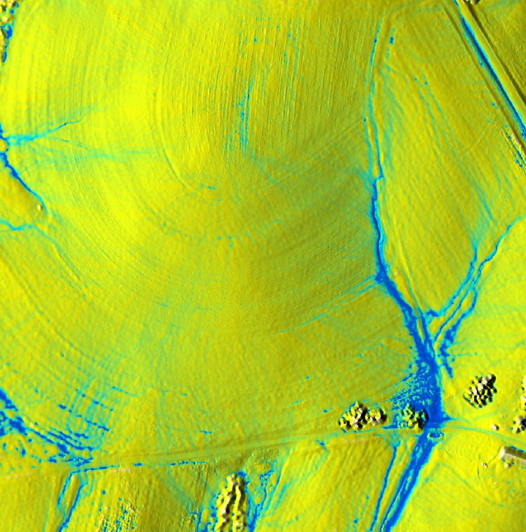
Spatially variable overlap
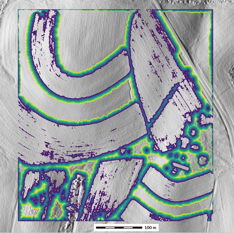
Bare ground UAS DSM is used to update lidar bare ground DEM using spatially variable overlap
Modeling overland flow
Microtopography captured at ultra-high resolution by UAS SfM poses special challenges to flow routing:
- real depressions are important features
- complex pattern of ponding, overflow of barriers is not supported by standard tools
- noisy surface requires robust algorithm
Path sampling method
Stochastic method for solving flow continuity equations
Flow over UAS mapped field
Crop surface creates barrier leading to artificial ponding
Flow over patched DEMs
Replacing crop surface by lidar bare ground: patching creates artificial flow pattern, smooth fusion improves accuracy of flow distribution
Example from assignment
Water flow on DSM created by simple patching vs. smooth patching
Example from assignment
Water flow on DSM vs. bare ground fused from UAS DSM and lidar DEM
What did we learn?
- evaluation and interpretation of differences between lidar and UAS SfM DEMs
- teachniques for smooth fusion of high resolution DEMs
- impact of fusion technique on overland flow modeling
Intro to Python in GRASS GIS
Motivation
What is scripting good for?
- running tasks and workflows repeatedly on many datasets
- sharing your workflow with colleagues
- making your work reproducible (for your own benefit)
Why Python?
- most widely used language in geospatial applications
- easy to learn
- active community, many libraries
Running Python in GRASS
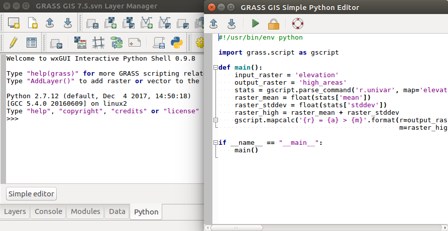
Python shell for one-line statements, editor for scripts
GRASS Python Scripting Library
- Enables to run GRASS GIS modules
- Import:
import grass.script as gs - run_command: most commonly used, for modules without text output, with raster/vector output
gs.run_command('g.region', raster='elevation') gs.run_command('r.neighbors', input='elevation', output='elev_smoothed', method='average', flags='c') - Compare to GRASS command line syntax:
g.region raster=elevation
r.neighbors input=elevation output=elev_smoothed method=average -c
GRASS Python Scripting Library
- read_command: used when we are interested in text output
gs.read_command('r.univar', map='elev_smoothed', flags='g')n=1142647 null_cells=207394 cells=1350041 min=110.196601867676 max=128.924560546875 ...
GRASS Python Scripting Library
- parse_command: used with modules producing text output as key=value pair
gs.parse_command('r.univar', map='elev_smoothed', flags='g'){'min': '110.1966018', 'max': u'128.9245605', 'cells': u'1350041', ...}
Allows convenient access to variable in dictionary:gs.parse_command('r.univar', map='elev_smoothed', flags='g')['range']18.72795867
GRASS Python Scripting Library
- write_command: for modules expecting text input from either standard input or file
gs.write_command('v.in.ascii', input='-',
                 stdin='%s|%s' % (635818.8, 221342.4),
                 output='view_point')
GRASS Python Scripting Library
- Other functions: calling r.mapcalc
gs.mapcalc("elev_strip = if(elevation > 100 && elevation < 125,
            elevation, null())")
