GRASS GIS 7 GUI intro
Note: The screenshots were done for GRASS GIS 7.0, there might be therefore slight differences for newer versions of GRASS.Start
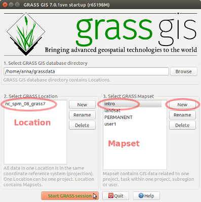
GRASS data structure
For this introduction we create new mapset intro to keep data organized.
Display
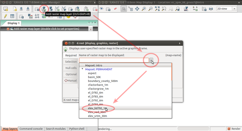
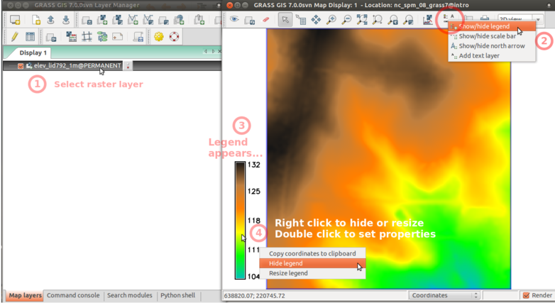
GRASS GUI: Add raster map elev_lid792_1m
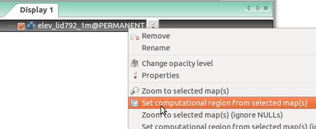
Set the computational extent and resolution of the mapset to match map elev_lid792_1m.
Computational region will be explained later.
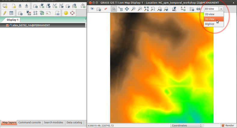
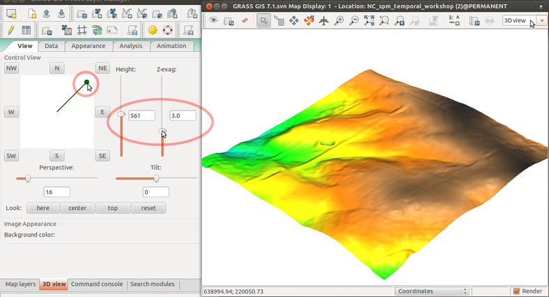
Display elevation in 3D view
Display elevation legend
GRASS modules
GRASS functionality is available through modules (tools). Modules respect following naming conventions:
| group | prefix | examples |
|---|---|---|
| general | g.* | g.list, g.remove, g.copy |
| raster | r.* | r.univar, r.neighbors, r.contour |
| vector | v.* | v.info, v.generalize, v.db.select |
| 3D raster | r3.* | r3.info, r3.to.rast, r3.colors |
| temporal | t.* | t.list, t.rast.aggregate, t.vect.univar |
| ... | ... | ... |
Finding and running a module
Type name or keyword in Search:
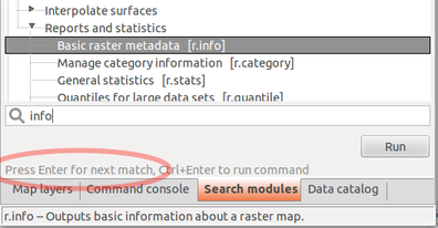
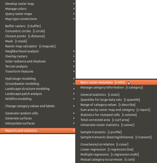
Raster > Reports and statistics > Basic raster metadata
Type beginning of command in Command console
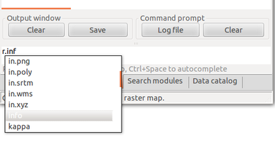
Command console supports auto-completion of maps and parameters.
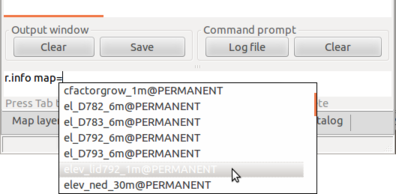
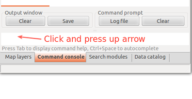
Browse command history using up and down arrows.
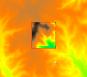
Region settings
Before we use a module to compute a new raster map, we must set properly computational region. All raster computations will be performed in the specified extent and with the given resolution.g.region -p north: 220750 south: 220000 west: 638300 east: 639000 nsres: 1 ewres: 1 rows: 750 cols: 700 cells: 525000
We can set it to match a raster map like this:
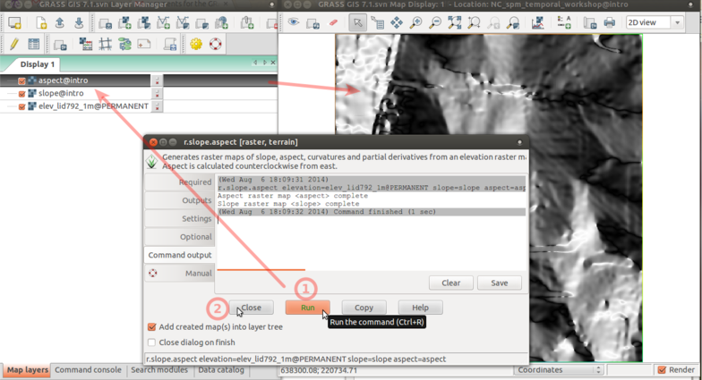
Running modules
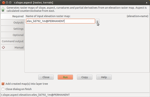
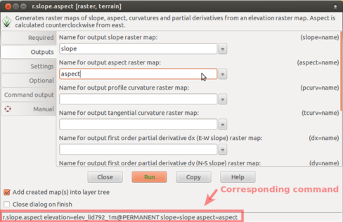
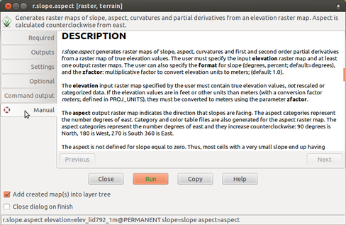
Module example: r.slope.aspect
Raster > Terrain analysis > Slope and aspect
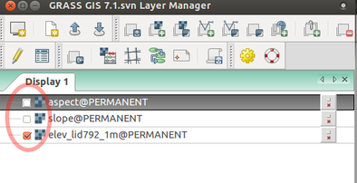
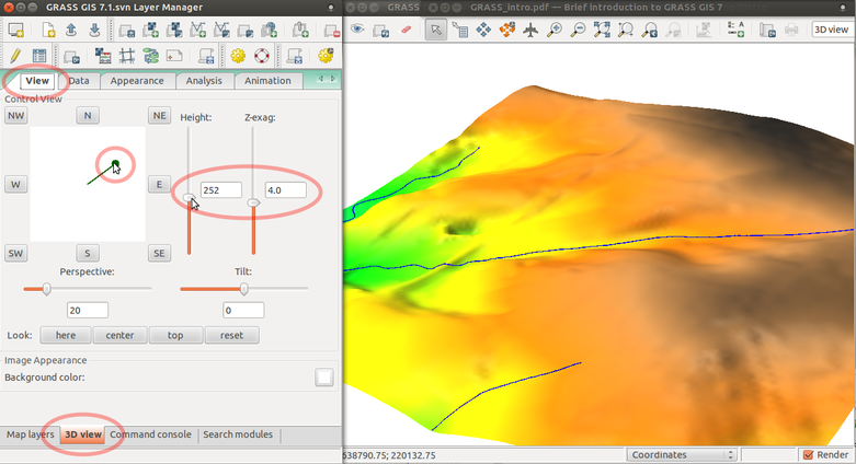
3D view
Uncheck newly created maps:
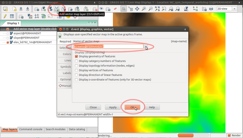
Add vector map streams:
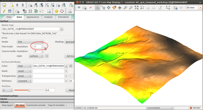
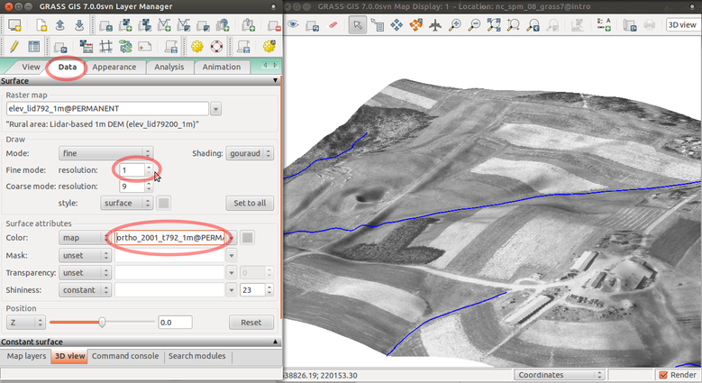
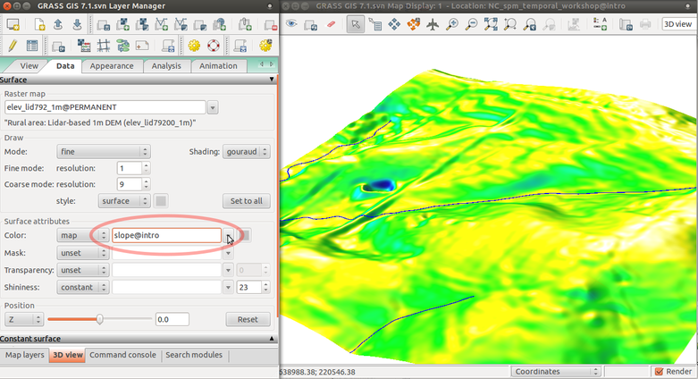
Set resolution and map draped over the surface:
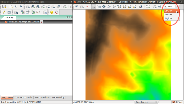
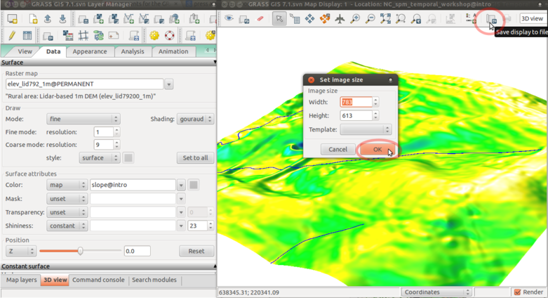
Save picture as TIF or PPM file and then quit GUI:
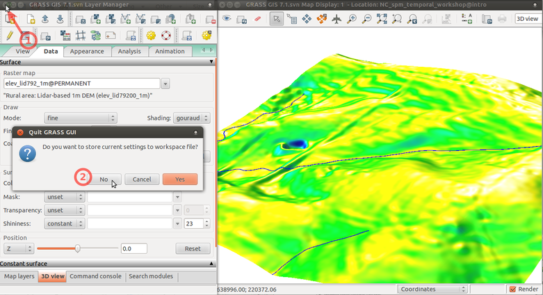
Quit GRASS session