Geostatistical simulations
Helena Mitasova, Anna Petrasova, Vaclav Petras
GIS714 Geosimulations NCSU
Learning objectives
- motivation for geostatistical simulations
- when to use spatial interpolation or geostatistical simulation
- geostatistical conditional simulations
- simulations for error propagation
- coupling GRASS and R for geostatistics
Problem formulation
In previous units we generated DEMs with simulated noise by adding a single realization of random values to a DEM with:
- uniform distribution
- Gaussian distribution
- distribution with spatial autocorrelation
- fractal
We then visualy evaluated the impact of different noise distribution on the flow pattern modeling and stream extraction.
Problem formulation
Patterns of flow accumulation from noisy DEMs:uniform, fractal, gaussian with spatial dependence
How to quantify uncertainty in the spatial pattern of the modeled variable due to uncertainty in elevation values?
Where is the high probability of a stream?
Problem formulation
- To quantitatively evaluate uncertainty in parameters derived from a DEM we can generate multiple realizations of a DEM by starting with different seed
- This approach does not take into account the spatial dependency of the elevation values in our data
- We can use geostatistical conditional simulation to generate multiple DEM realizations and use them to estimate error propagation in derived variables
Computing the surface model
From scattered points (red) to a regular grid (blue)
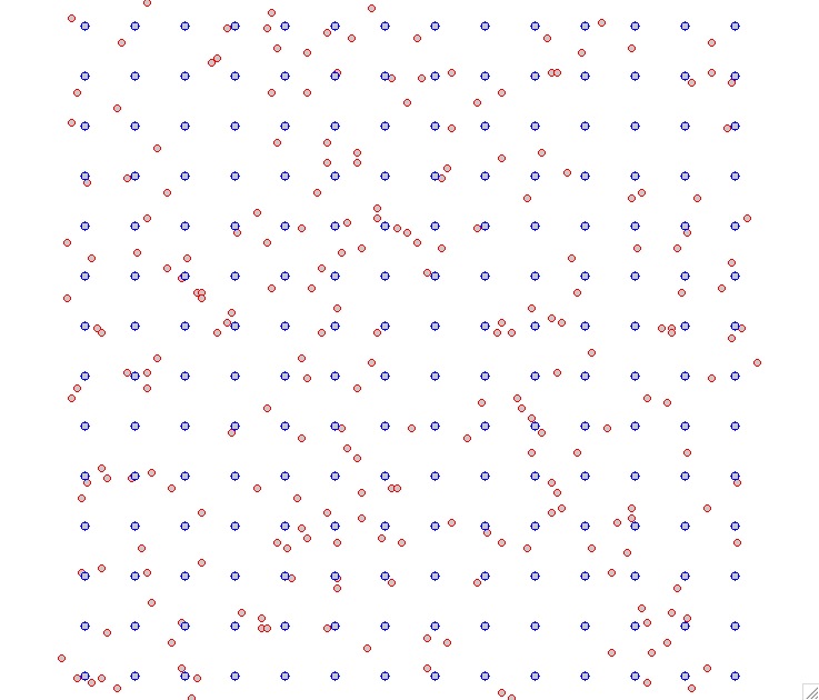
The scattered points can be the original measured data or a random sampling of a given raster (e.g. DEM)
Computing the surface model
Derive model of spatial distribution of a variable based on a limited set of discrete scattered observations:
- if the measured data capture features of the distribution at the level of detail needed
for the application we can use interpolation
See GIS582 Spatial interpolation topic - if the measured data are limited and we know statistical properties of the distribution, we can use simulation
Spatial interpolation
Given $m$-points $(x_i, y_i, z_i), i=1,m$
find such continuous function $F(x,y)$ that for each $i=1,m$
$$z_i=F(x_i,y_i)$$
$$ F(r) = T(r) + \sum_i^m \lambda_i R(r,r_i) $$
then use $F(r)$ to compute $z$ at unsampled grid points
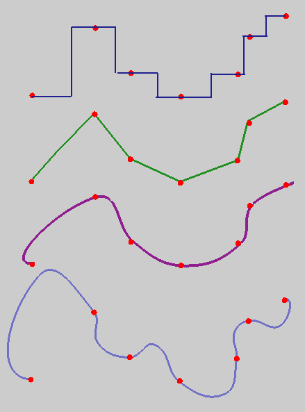
Spatial interpolation
The problem of finding $F(x,y,)$ that passes through (or close to) the given points does not have a unique solution:
Interpolation with radial basis functions
Variational approach is based on minimizing:
- deviations from the given points
- smoothness seminorm or roughness penalty
Radial basis functions: multiquadrics, splines
Physics-based interpretation: spline interpolation function is a thin flexible plate with tunable bending energy, formally equivalent to universal kriging
Spline tension rescales distances, it has similar effect to shortening range in kriging or decreasing the distance weight exponent in IDW
Spline: tension
Tension controls the stiffness of the plate:- high tension: soft rubber sheet, short range
- low tension: stiff steel plate, long range
Spline: tension t=160

Spline: tension t=40
Spline: tension t=10
Spline: tension
High tension, short range of influence, soft rubber sheet, results in a rough surface with a peak or pit in each data point
Low tension, long range of influence, stiffer steel plate, results in a smoother surface with possible overshoots.
Note that tension is inverse of stiffness
Spline: smoothing
Smoothing controls the deviation from the data points, large smoothing results in trend surface $T(x,y)$
Reduces overshoots, noise, improves numerical stability, can be applied to individual points
Spatial interpolation
Example of using smoothing spline with tension:
Univariate spline applied to wastewater monitoring of COVID-19 virus
Note: Spline interpolation methods are based on deterministic simulations of a thin flexible sheet, but they are also equivalent to universal kriging with the covariance function determined by a roughness penalty see Mitas 1999
Geostatistical approach to interpolation
General equation$$ F(r) = T(r) + ∑ λ_j R(r,r_j) \; j=1,m $$
- $r = (x,y)$ is location of a unsampled grid point,
- $r_j=(x_j,y_j$) is location of a measured point
- $T(r)$ is trend (low order polynomial),
- $λ_j$ are coefficients
- $R(r,r_j)$ is a model variogram (function of distance between unsampled and measured point)
The coefficients $λ_j$ are found by solving a system of $m$ linear equations
Geostatistical approach
We assume that the points that are close to each other have smaller differences in measured values than the points that are farther appart
- Model variogram $R(r,r_j)$ is derived by fitting a suitable function to empirical variogram
- empirical variogram is derived from data as
$$ \gamma (h) = (1/m_h) ∑[z(r_i) - z(r_j)]^2 \; i=1,…, m_h $$
which is mean square of differences in measured values $z$ for points that are separated by a distance $h$ (with some tolerance defining the size of histogram bin)
Many model functions can be used: spherical, exponential, Gaussian, …
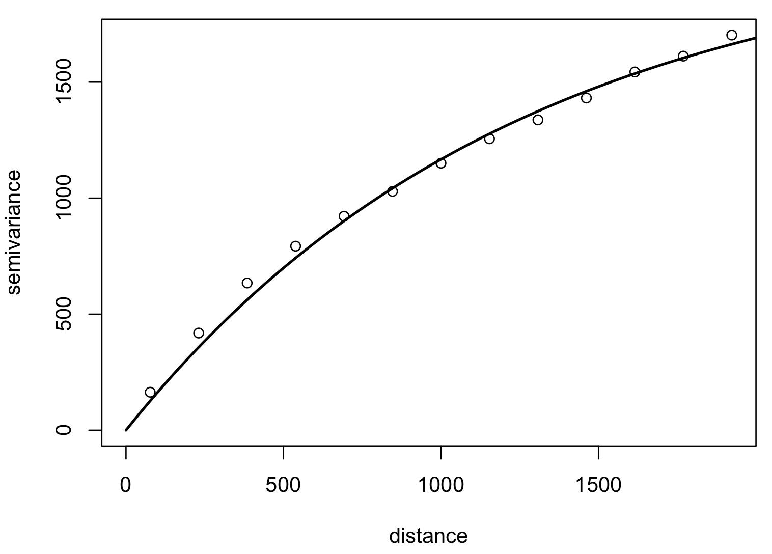
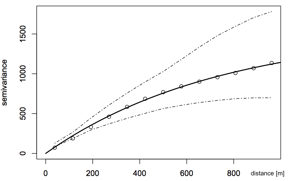
Experimental variogram
Given set of elevation points and derived experimental variogram

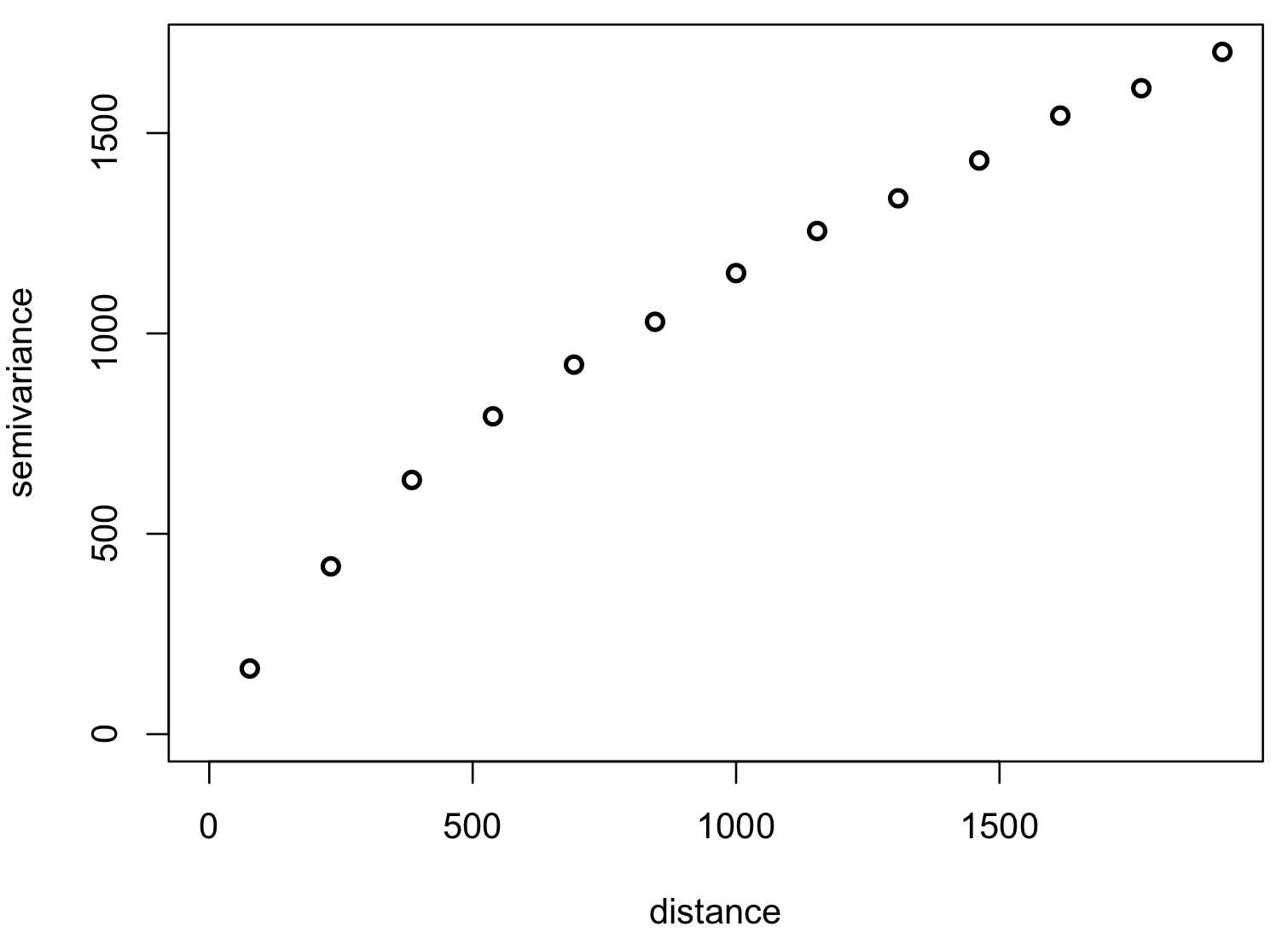
Maximum distance is 2000 m, histogram bin is ~150m. Adapted from A Practical Guide to Geostatistical Mapping by T. Hengl.
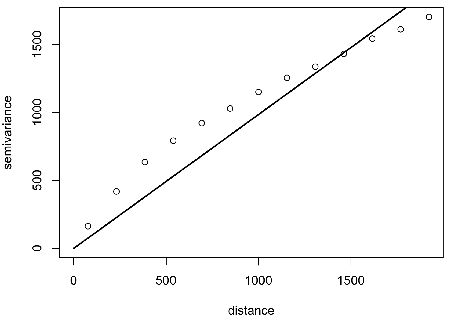
Model variogram
Optimized fit of a suitable function to empirical variogram: linear
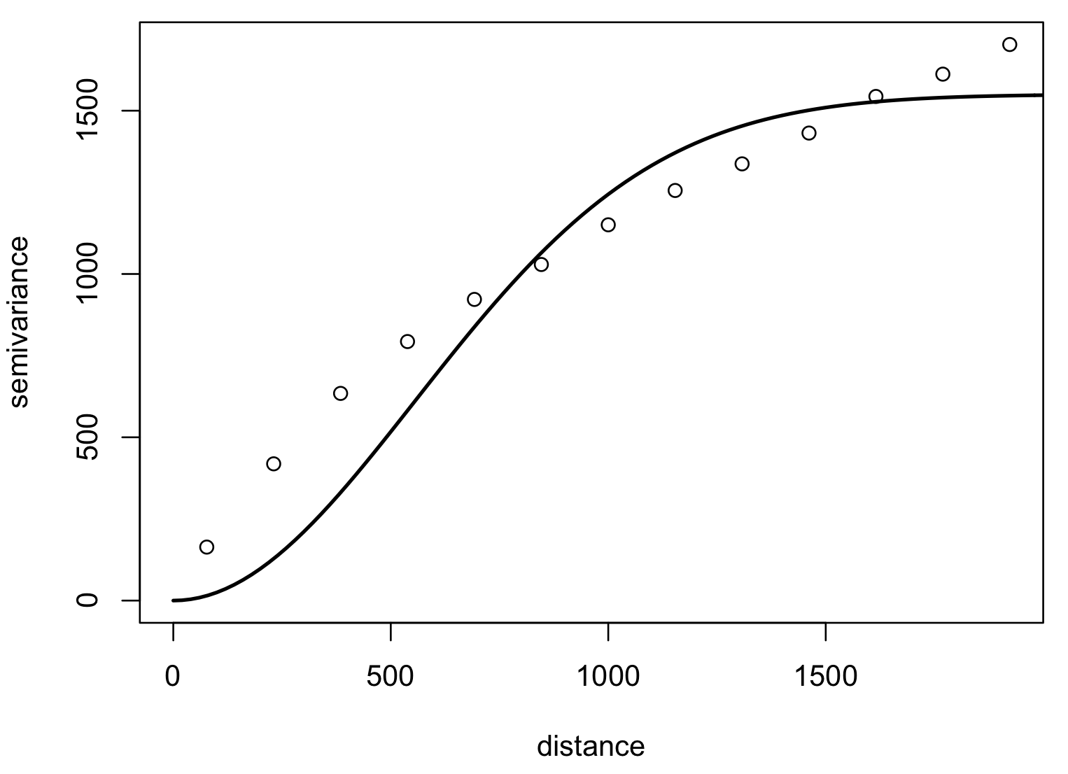
Model variogram
Optimized fit of a suitable function to empirical variogram: gaussian, spherical
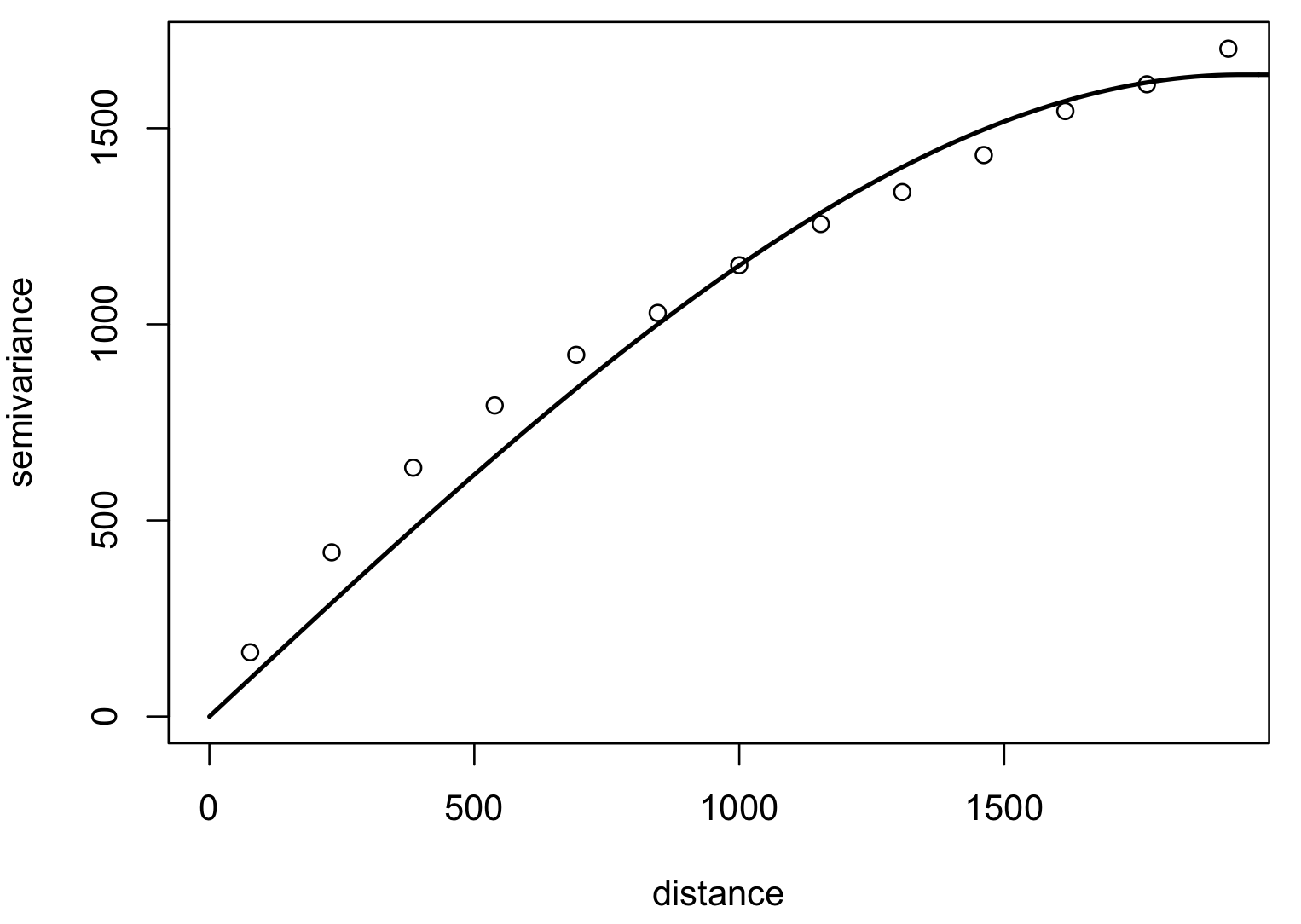
Model variogram
Optimized fit of a suitable function to empirical variogram: exponential, Matern

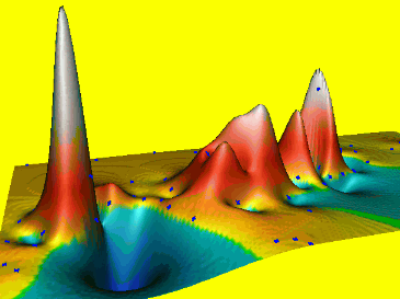
Kriging: Interpolated surface
Single realization of a DEM interpolated with kriging using Matern model variogram
Interpolation or simulation?
- Interpolation: we use $F(x,y)$ to estimate values at unsampled locations resulting in a single realization of the surface
- Simulation: we use $F(x,y)$ to condition our simulation of a more complex surface than what we could generate using interpolation from the given points
Geostatistical simulations
- modeled spatial distribution is complex
- limited number of samples is available - interpolation does not capture the complexity, result is too smooth
- we have some knowledge of statistical properties of the modeled distribution
- we generate many realizations of the surface using the given statistical properties
- the realizations are used to compute the simulated distribution mean and uncertainty maps
Applications
Observations where sampling is limited:
- subsurface: reservoir modeling in petroleum industry, mining, soil properties, groundwater pollution
- surface: variables not detectable by RS, e.g. some pollutants
- generate multiple realizations of modeled distribution for uncertainty propagation studies
Analyze the input data
- input: sparse, scattered point measurements
- analyze the data for normality (compute histogram)
- apply transformation if needed to get normal distribution (log or Box-Cox transform)
- compute experimental and model semivariogram
- define spatial extent and resolution of resulting grid
Generate one grid realization
Workflow for Gaussian Sequential Simulation- assign data points to closest grid cell (nn binning)
- select random unsampled grid cell and compute kriged estimate + random residual to get simulated value using the neighboring given points
- use "random path" to define order of empty grid cells to be simulated
- at each new unsampled grid cell use the nearby given points and previously simulated values to compute the simulated values
nn binning assumes that the grid cell size is smaller than the min distance between points, otherwise we would need to aggregate some points, e.g. using mean
Gaussian Sequential Simulation
- Each realization starts with a different seed
- Compute hundreds or thousands realizations
- Result: mean simulated values grid and standard deviation grid
Error propagation application
- Given a set of elevation points quantify uncertainty in the stream position derived from DEM computed from these points while taking into account DEM errors.
- Assignment Example from A Practical Guide to Geostatistical Mapping by T. Hengl.
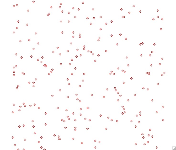
Elevation data analysis
Distribution of all points, points with non-integer $z$ values and points with $z=180$
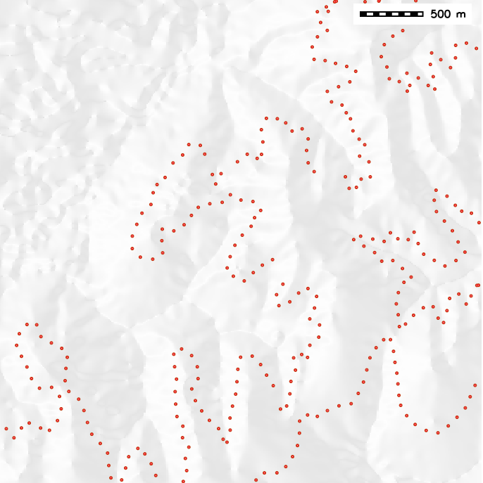
Our data set includes points along contour lines combined with scattered points along ridge lines and valleys and in the floodplain.
Elevation data analysis
Given points assigned to nearest 10m grid cell and a related histogram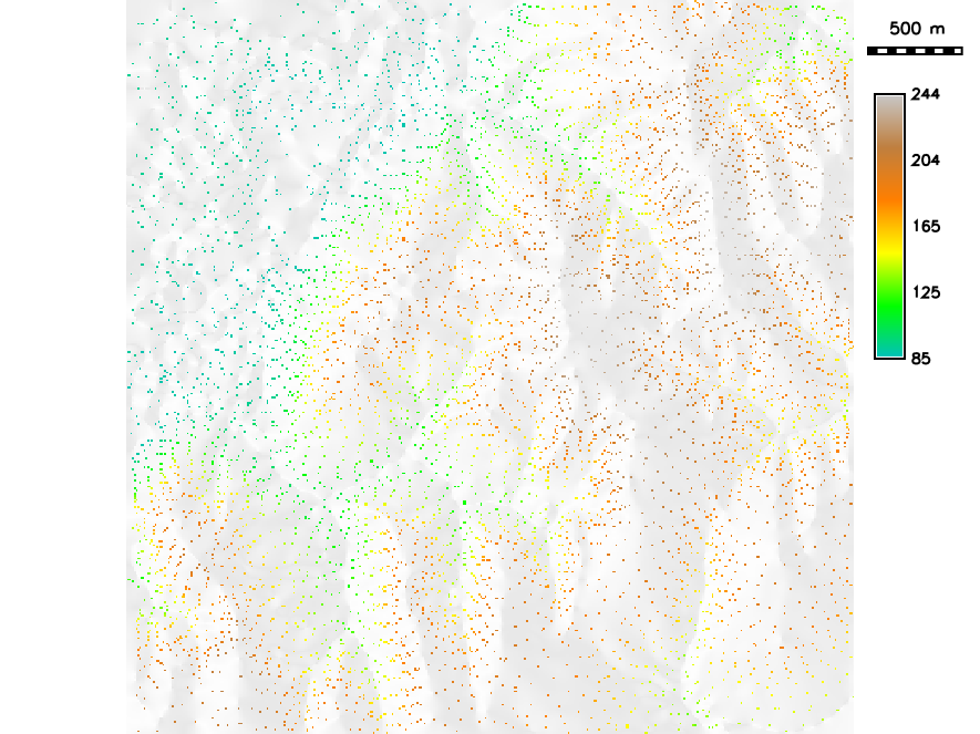
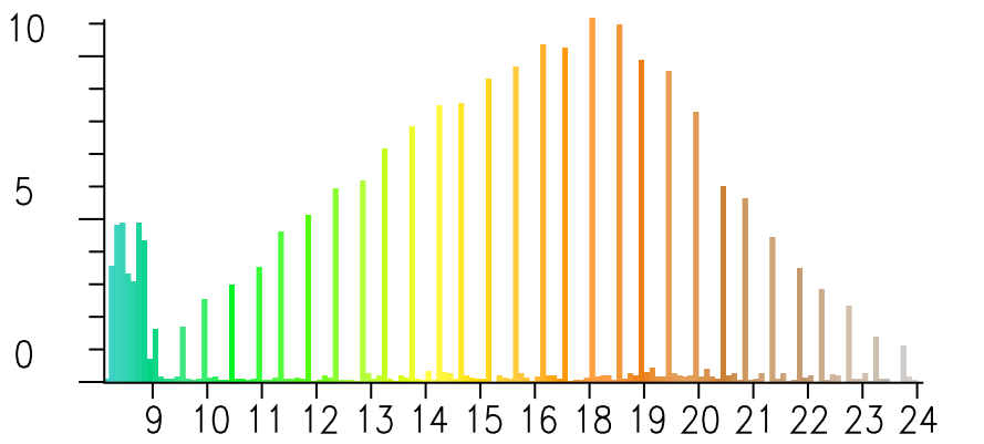
Note that for $z>90m$ there are many points with values at 5m intervals while there are very few points with values in-between, reflecting the dense sampling along contours. Histogram $x$ is in tens of meters and $y$ in hundreds of cells
Smooth DEM interpolation
DEM interpolated by spline with tension and its histogram 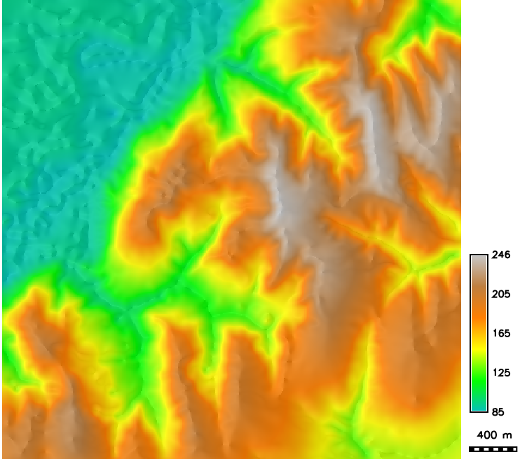
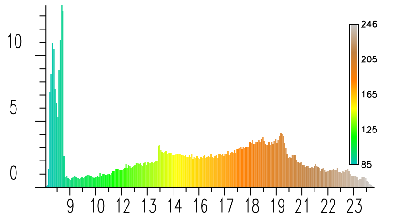
Note that the histogram of interpolated DEM is quite different from the histogram from the data
Elevation data analysis in R
Plot distribution for 20% and 80% of sub-sampled points
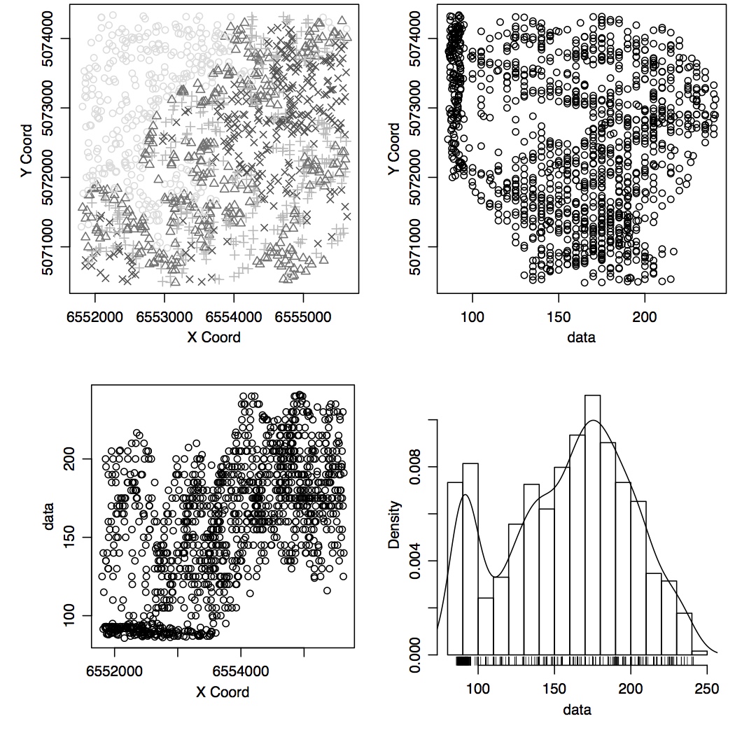
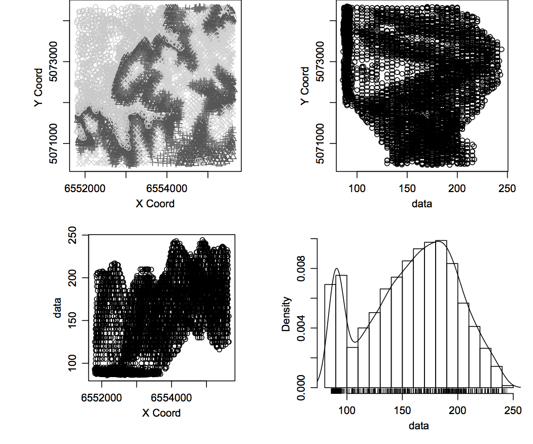
Note that the histogram is different from the previous two: it does not capture
the difference between the number of points on contours and the scattered points because
of aggregation in smaller number of histogram binns (20 in R versus 255 in GRASS).
Elevation data analysis
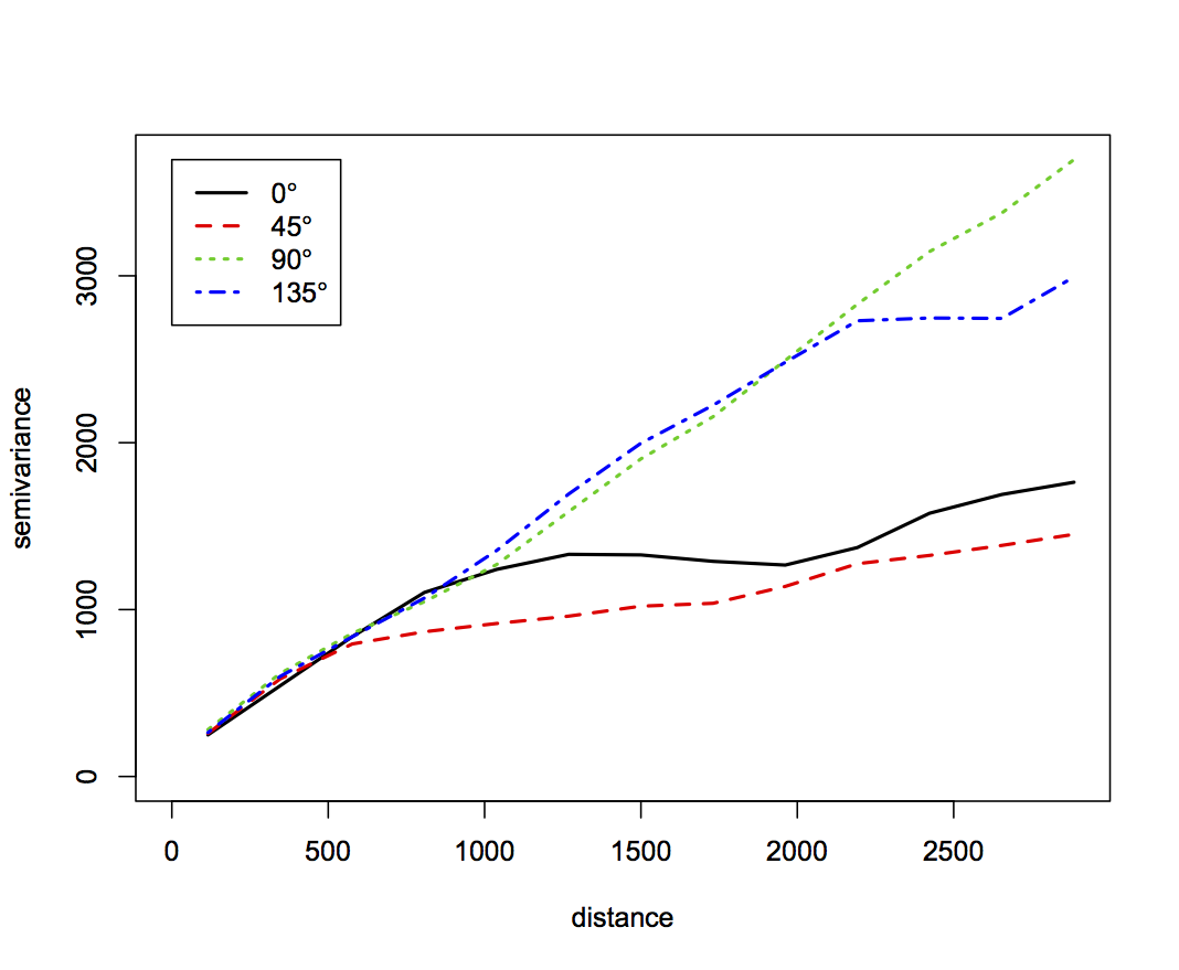
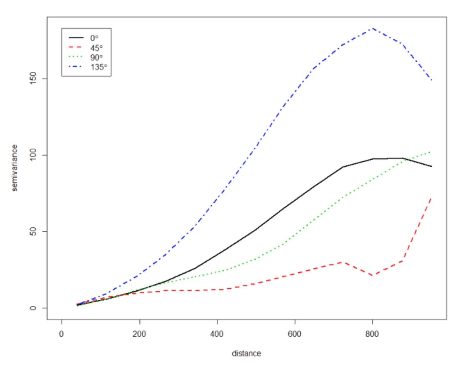
- Anisotropic experimental variogram from given data using 20% and 80% sub-sampled points
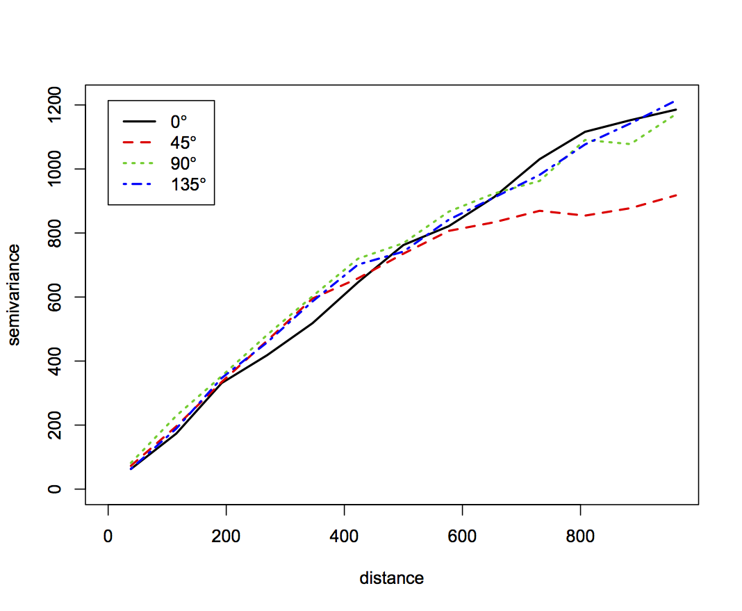
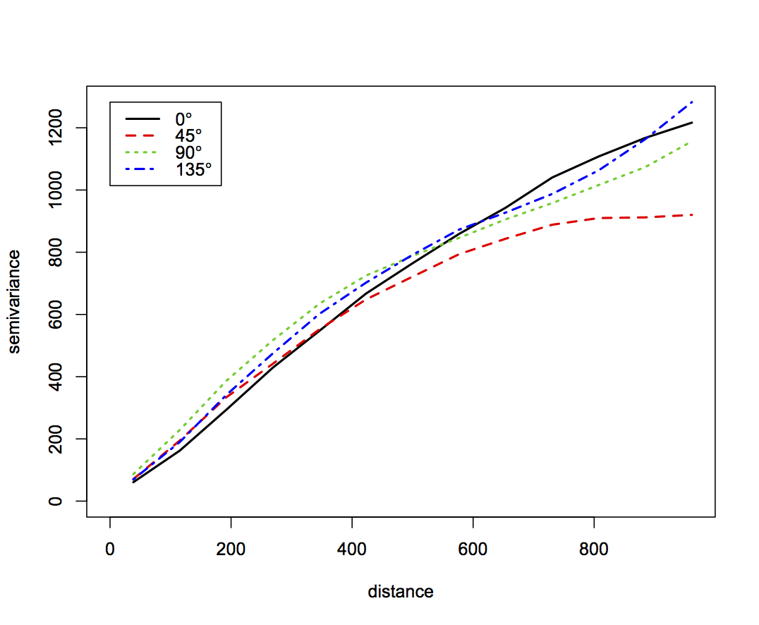
The 80% subsample leads to a smoother variogram, but as little as 20% points captures the characteristics of spatial dependence (autocorrelation). Note slight anisotropy in 45 degrees direction (direction of floodplain edge has lower sill)
Elevation data analysis
- Anisotropic experimental variogram for 1000m and 3000m maximum distance
The variogram shows stronger anisotropy for distances over 1km. When applying GSS, the variogram is used locally (10s-100s of meters) so we can use an isotropic variogram model
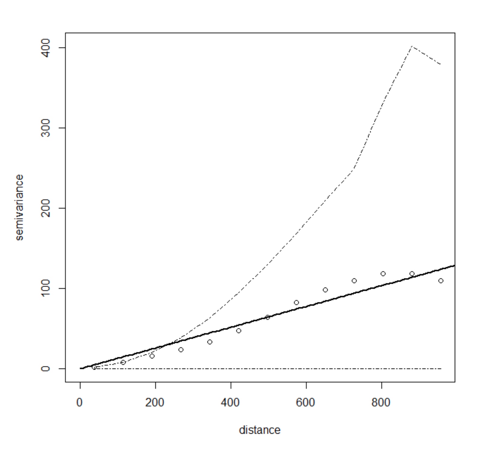
Model variogram
- Matern model variogram with smoothing is needed to avoid DEMs with artifacts - see Hengel et al.
- Model variogram is fitted using the weighted least squares, shown with confidence bands
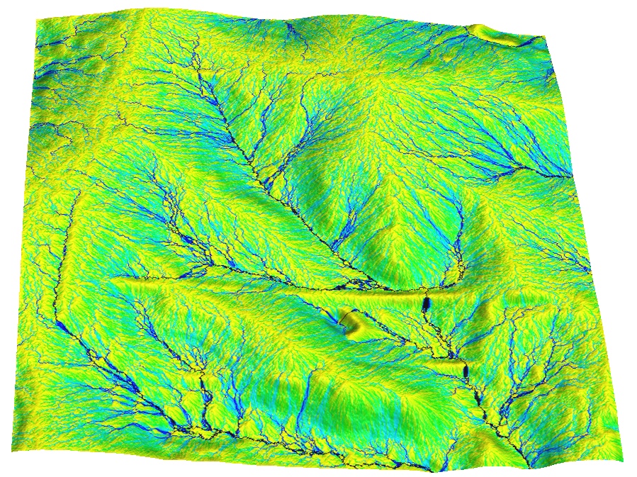
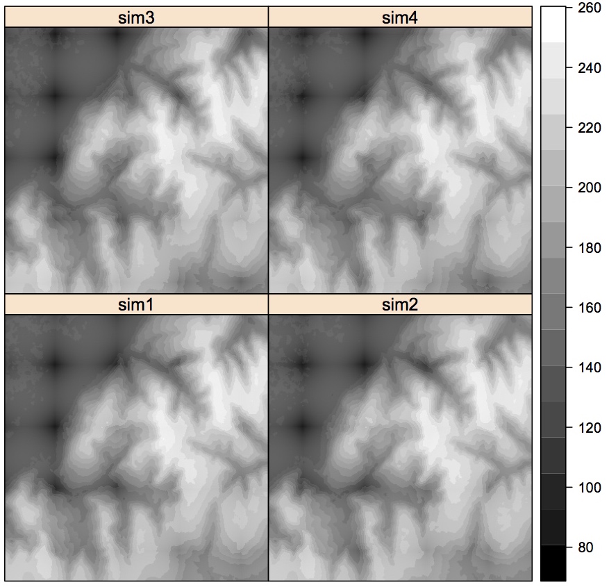
Conditional simulation of DEMs
- Four out of 100 realizations of a DEM in R
Note the JPEG effect(?) in the BW image at low elevation
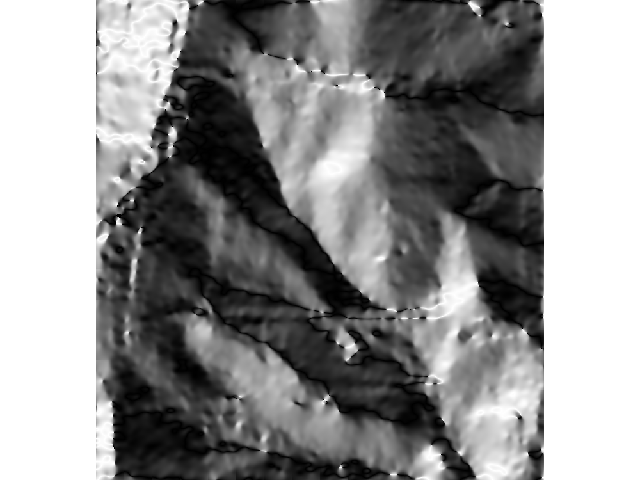
Conditional simulation of DEMs
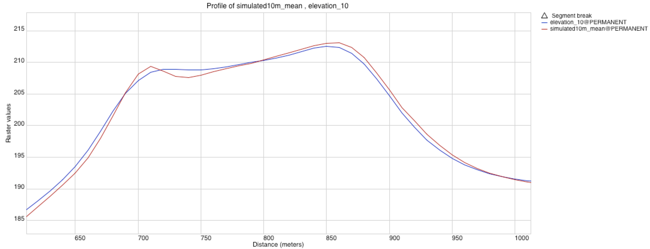
- One of 100 DEM realizations and the mean DEM
The white spots indicate locations where the simulated DEM is above or below the range of interpolated DEM, but within the range of given data.
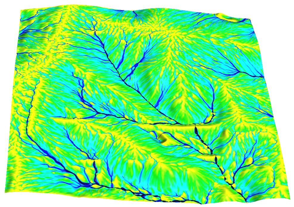
Conditional simulation of DEMs
- Mean simulated DEM and its standard deviation map
Standard deviation is much higher in the floodplain and along edges, reflecting insufficient sampling. This is already indicated by comparing the histogram from the data and histogram from the interpolated DEM.
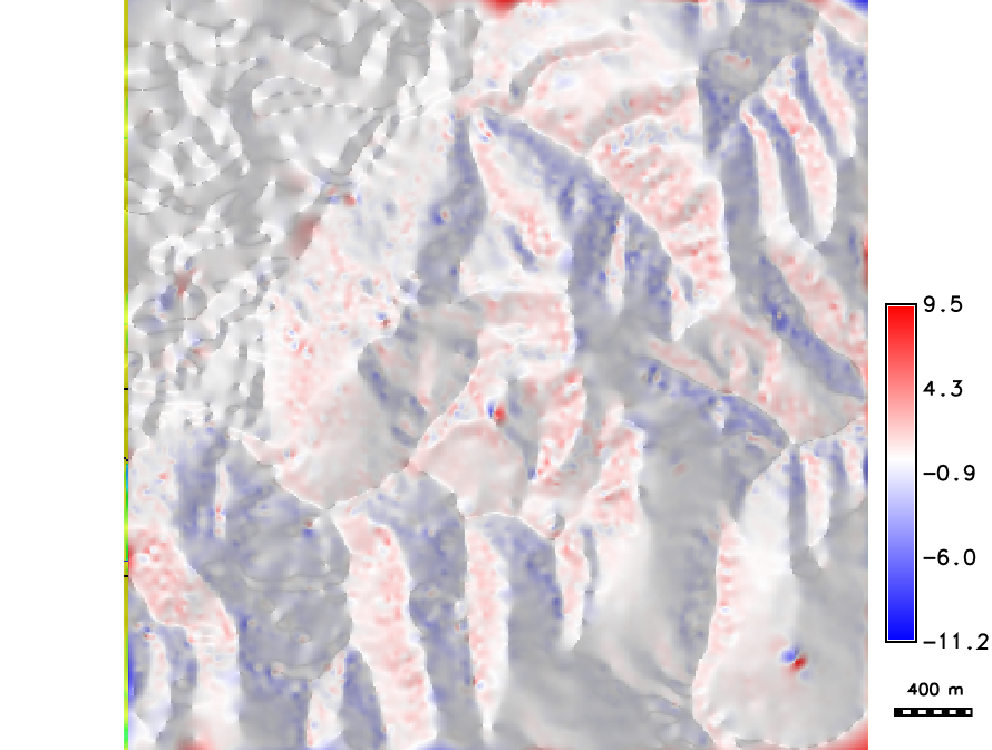
Interpolated and simulated DEMs
- Difference between DEM interpolated in GRASS and DEM simulated in R indicates shift of approx 1 grid cell. Problem during export/import? Test the fix
Stream extraction uncertainty
How does the error in DEM influence the uncertainty in the location of extracted streams?
- derive $n$ stream networks from $n$ DEM realizations
- compute per-cell count $m$ of stream presence from $n$ derived stream networks
- derive probability of stream location at each grid cell as $p = m/n$
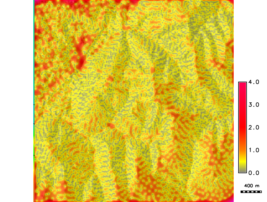
Then propagated error of extracted streams is $$e = -(1-p) \ln(1-p) - p \ln(p)$$
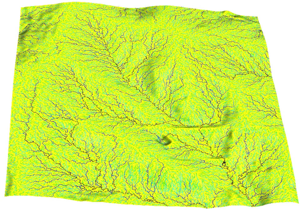
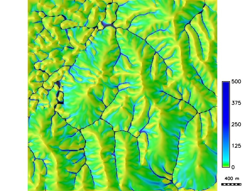
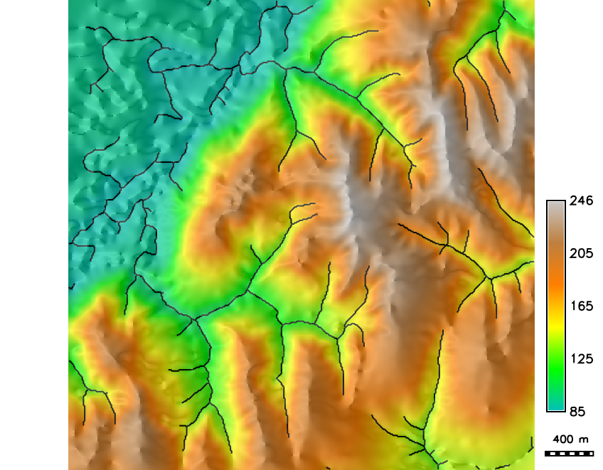
Streams derived from smooth DEM
Flow accumulation and streams derived from the smooth DEM using D8-MFD-LCP method and threshold 300 of 10m resolution cells: deterministic result
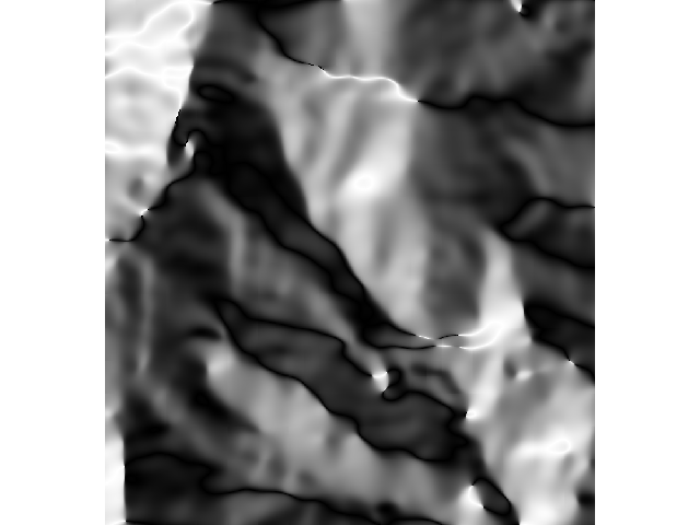
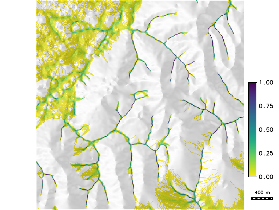
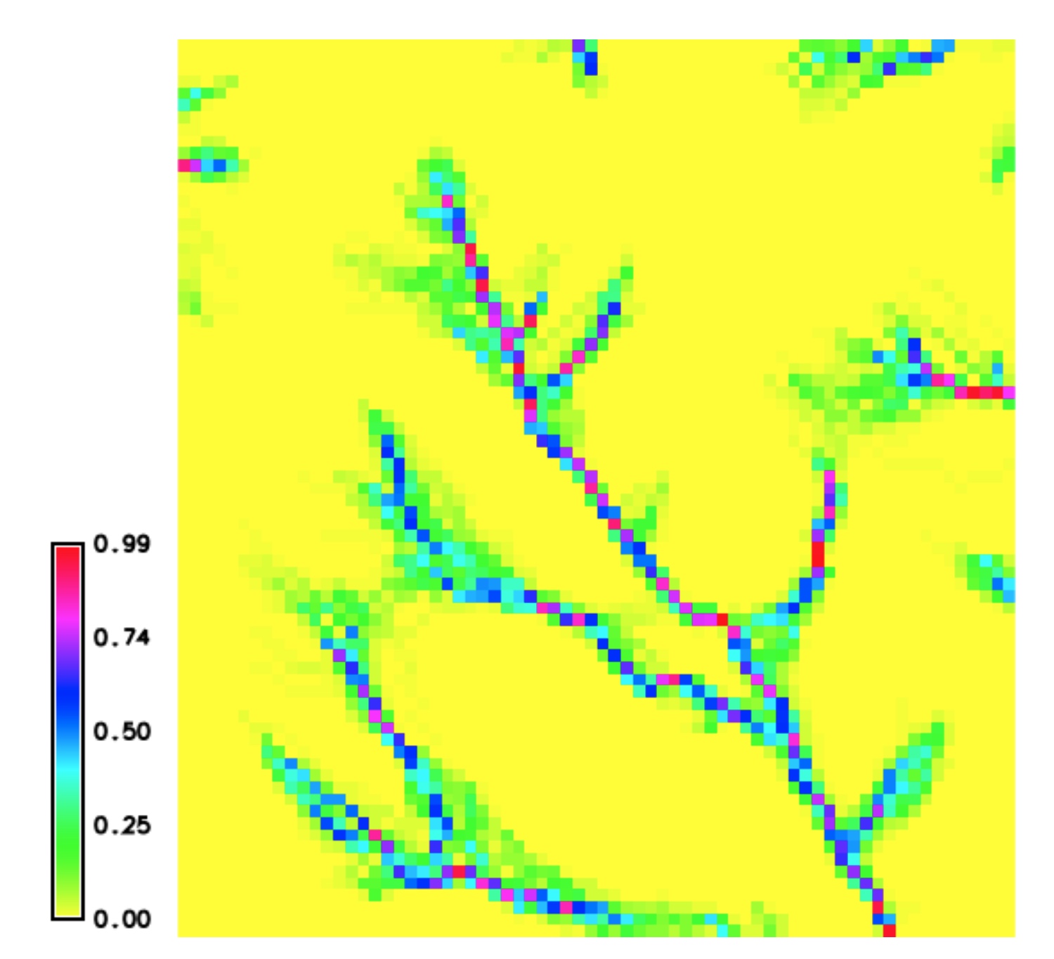
Stream probability map
Stream probability map with $p>0$ and the probable streams with $p>0.5$
Examples of Applications
The approach can be applied to estimate uncertainty and error propagation for other analysis and modeling problems using the $n$ DEM realizations:
- flood extent prediction
- viewshed mapping and visibility analysis
- cast shadows and solar radiation
- least cost path
- soil erosion and mass transport
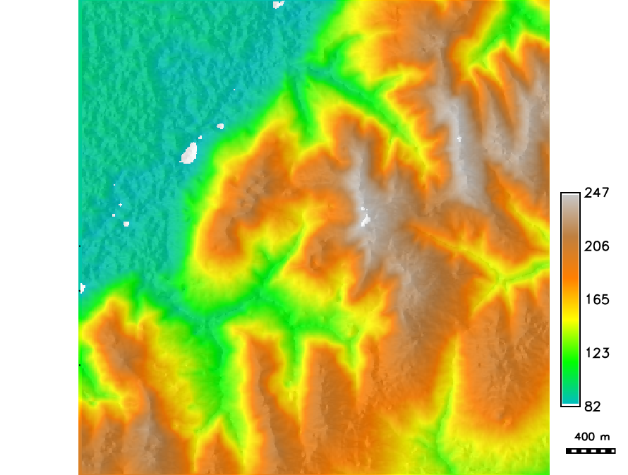
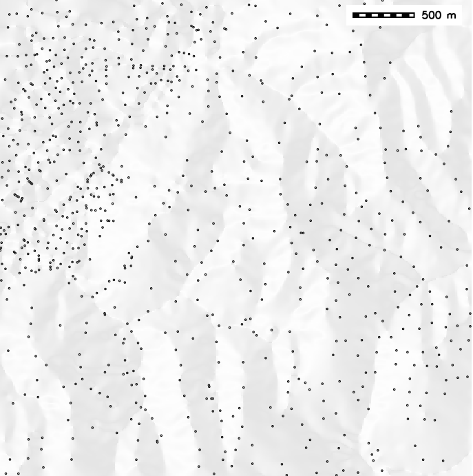
Elevation data analysis
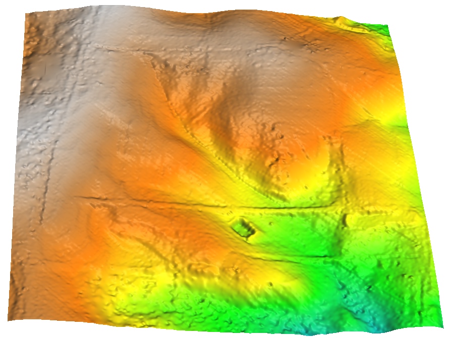
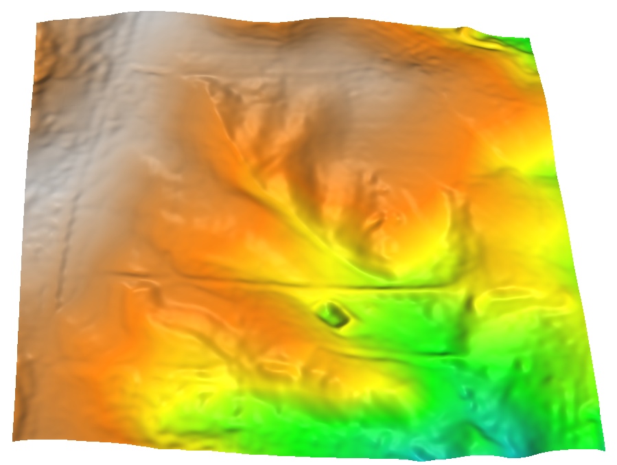
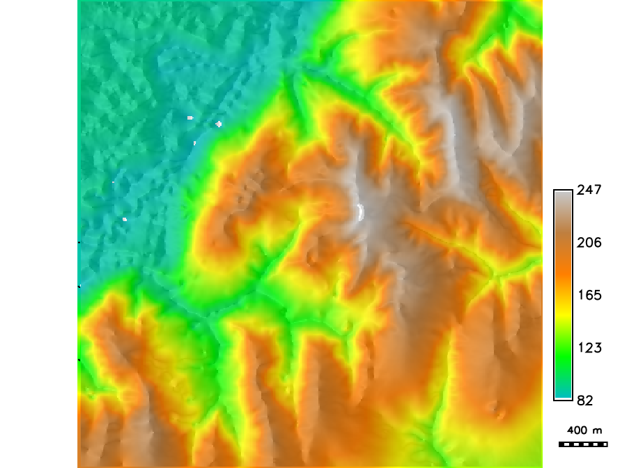
Lake Wheeler SECREF DEM and plot of given points
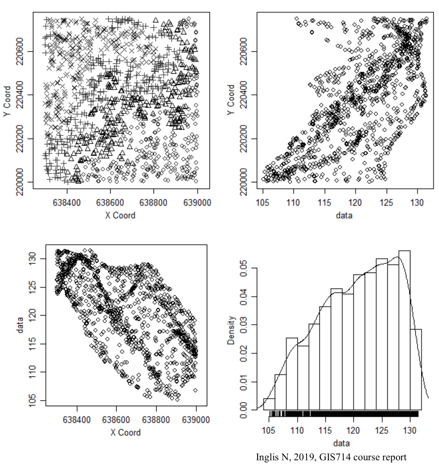
Elevation data analysis
- Anisotropic experimental variogram from given elevation data
- Matern variogram model with smoothing parameter
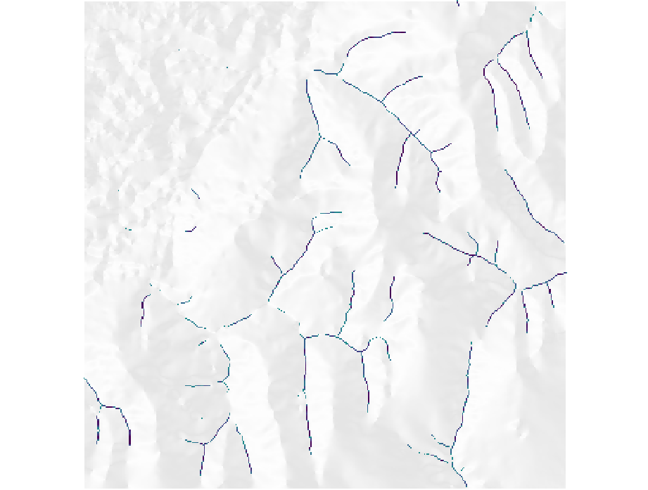
Generate 100 DEMs (2m resolution) and extract streams from each
Inglis N., 2019, GIS714 course assignment report.
Stream probability map
Inglis N., 2019, GIS714 course assignment report.
Resources
Spatial Statistics course at NCSU, Dr. Brian Reich
See supplemental material, especially Hengl et al.: Geomorphometry (Chapter 5 by Temme et al), and Hengl: A Practical Guide to Geostatistical Mapping