Soil erosion and deposition modeling

Theoretical background

Helena Mitasova

Landscape potential for soil erosion and deposition can be estimated and mapped using Unit Stream Power Based Erosion Deposition model (USPED). The concept was proposed by Moore and Burch (1986) as a model of sediment transport limited case of erosion/deposition and implemented in GIS by Mitasova et al. (1996) as part of SERDP project (REF).

USPED combines the Universal Soil Loss Equation USLE parameters and upslope contributing area to estimate sediment flow and then erosion and deposition rates are computed as change in sediment flow in the direction of steepest slope.

USLE

The general equation for USLE is

E = R.K.L.S.C.P

where
E is average annual soil loss in ton/(acre.year) = 0.2242kg/(m2.year) = 2.242ton/(ha.year),
R is rainfall factor in (hundreds of ft-tonf.in)/(acre.hr.year) = 17.02(MJ.mm)/(ha.hr.year),
K is soil erodibility factor in (ton acre.hr)/(hundreds of acre ft-tonf.in) = 0.1317(ton.ha.hr)/(ha.MJ.mm),
LS is a dimensionless topographic (length-slope) factor,
C is a dimensionless land cover factor, and
P is a dimensionless prevention measures factor.

The modified 3D topographgic factor LS3D, representing topographic potential for erosion at a point on the hillslope, is a function of the upslope contributing area per unit width and the slope angle:

LS = (m + 1) (U/22.1)^m (sin β/0.09)^n

where
U is the upslope area per unit width (measure of water flow) in meters (m^2/m),
β is the slope angle in degree,
22.1 is the length of the standard USLE plot in meters,
0.09 = 9% = 5.15◦ is the slope of the standard USLE plot.
The values of exponents range for m = 0.2 − 0.6 and n = 1.0 − 1.3, where the lower values are used for prevailing sheet flow and higher values for prevailing rill flow.

USPED model

We further modify the LS3D factor to represent topographic component of sediment transport capacity of overland flow LST:

LST = U^m.(sinβ)^n

and then sediment flow T at sediment transport capacity is estimated as:

T = R.K.C.P.U^m.(sinβ)^n

where
R, K, C, P, U, β are the same as in modified USLE, and U, β are not normalized, because
T is an estimate of sediment flow [kg/(m.s)] or [ton.m/(ha.year)] = [ton/(10000m.year)], (rather than soil loss E [kg/(m2.s)]).

The net erosion/deposition D is then computed as a divergence of sediment flow (change in a 2D field representing sediment flow in the direction of elevation surface gradient):

D = ∇ · (T s0) = ∂(T cos α)/∂x + ∂(T sin α)/∂y

where
α in degrees is the aspect of the terrain surface (direction of flow). We get D in [kg/(m2s)] by dividing T [kg/(ms)]/dx[m] or T [ton/10000m.year]/dx[m] = D[ton/(10000m2.year)] = D[(ton/ha.year)]

To make the equation easy to implement in any GIS with basic terrain analysis support, the erosion/deposition equation can be rewritten using the following relationship between partial derivatives and surface slope β and aspect α:

∂z/∂x = tan β . cos α ∂z/∂y = tan β . sin α

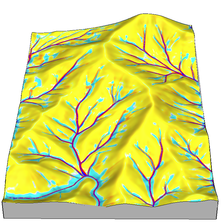
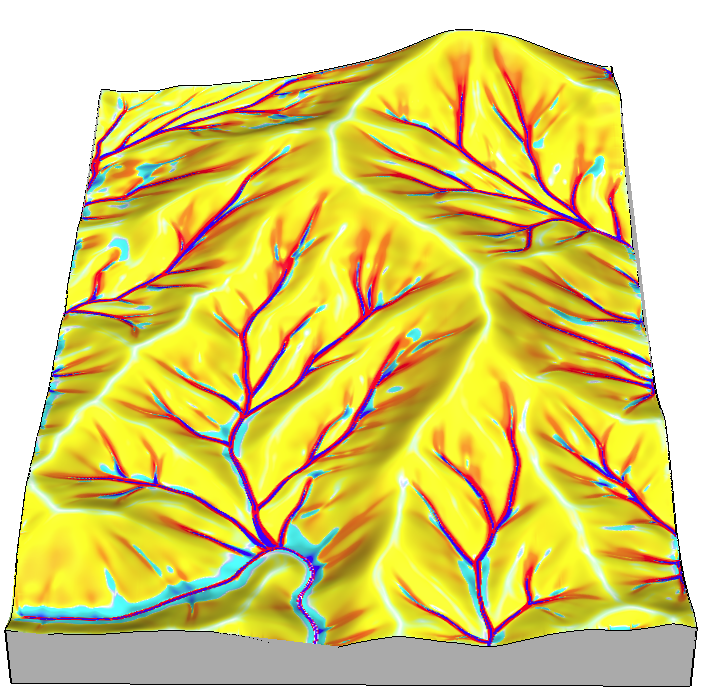
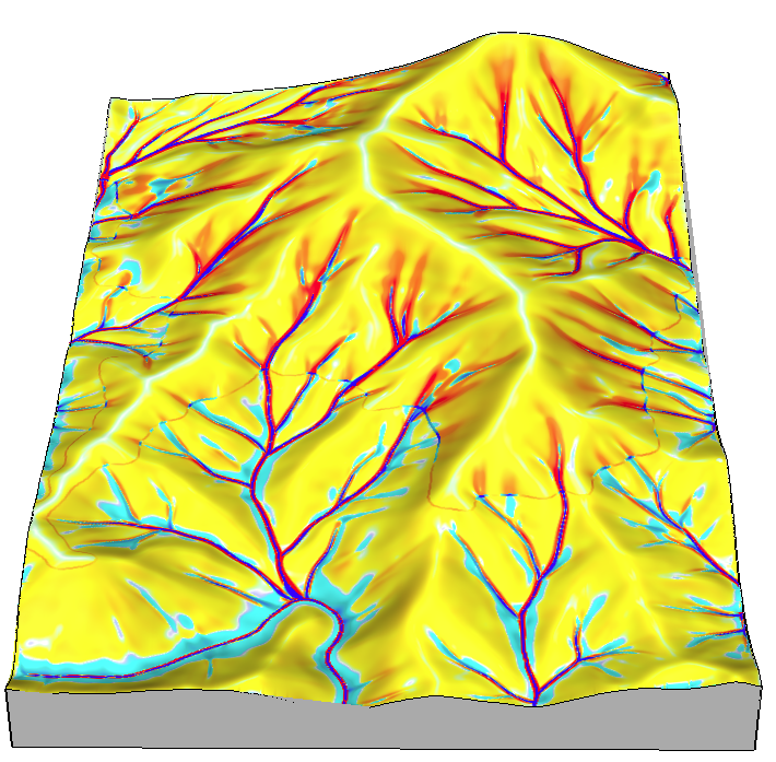
The exponents m, n control the relative influence of water and slope terms and reflect the impact of different types of flow. The typical range of values is m = 1.0 − 1.6, n = 1.0 − 1.3, with the higher values reflecting the pattern for prevailing rill erosion with more turbulent flow when erosion sharply increases with the amount of water. Lower exponent values close to m = n = 1 better reflect the pattern of compounded, long term impact of both rill and sheet erosion and averaging over a long term sequence of large and small events.