Assignment 2C
Processing the same imagery in WebODM
Task
Process the Assignment 2B photographs, camera positions, and ground control points in WebODM, the free and open source drone mapping software (WebODM contributors 2026), and compare the orthomosaic and DSM with the ones you produced in Agisoft Metashape. Same imagery, same control, different software: the differences you find are the software’s, not the flight’s.
Software
WebODM 3.2 is an independent open source project (since April 2026 at github.com/WebODM). Install it one of these ways:
Windows or macOS: download the free installer from webodm.org. The installer bundles everything, including the Docker backend on macOS. Windows 10 or newer with a 64-bit CPU; macOS 13 or newer, Apple silicon supported.
Linux: install Docker and Git, add yourself to the
dockergroup (sudo usermod -aG docker $USER, then log out and in), and rungit clone https://github.com/WebODM/WebODM --config core.autocrlf=input --depth 1 cd WebODM ./webodm.sh start./webodm.sh stopstops it and./webodm.sh updateupdates it.Memory: 8 GB RAM is the minimum and handles about 100 images, which covers this data set; 16 GB is recommended. 20 GB of free disk.
No suitable laptop? WebODM Lightning processes in the cloud from the same interface; it is a paid service with a small free allowance.
The OpenDroneMap organization sells an installer called “OpenDroneMap Desktop”. It is a different, older product. The WebODM installers are free.
Once started, open http://localhost:8000 and create the administrator account on the first visit. See the WebODM documentation for troubleshooting.
Data
- Download the data if you no longer have it from Assignment 2B: 78 photos, the flight log, and the coordinates of 3 GCPs.
- Two files prepared for WebODM, explained below:
- geo.txt: the camera positions in WebODM’s image geolocation format
- gcp_seed_epsg32617.txt: the three GCP coordinates in WGS84 UTM 17N, in the layout the GCP interface reads (also available in latitude and longitude as gcp_seed_epsg4326.txt)
Why geo.txt
The Trimble UX5 does not write GPS coordinates into the photos; the positions live in the flight log. Metashape imported the log directly. WebODM reads camera positions from the photos’ EXIF, and when there are none it accepts an image geolocation file named geo.txt: a header with the coordinate system, then one line per photo with the file name, longitude, latitude, height, and optionally yaw, pitch, and roll.
EPSG:4326
DSC06168.jpg -78.69809128 35.72773663 179.49 0.147352 0.0137609 -3.05065
DSC06169.jpg -78.69807484 35.72753443 177.82 0.0312571 -0.0901053 -3.09326
The provided file was generated from 2016_09_22_sample.txt with a few lines of Python. File names are case sensitive: the log says .JPG, the files are .jpg.
import csv

with open("2016_09_22_sample.txt") as log, open("geo.txt", "w") as geo:
    geo.write("EPSG:4326\n")
    for r in csv.DictReader(log):
        name = r["name"].replace(".JPG", ".jpg")
        geo.write(f"{name} {r['longitude']} {r['latitude']} {r['height']} "
                  f"{r['yaw']} {r['pitch']} {r['roll']}\n")
Stage 1: Project and ground control points
Create a project
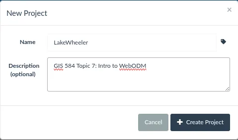
On the dashboard click Add Project at the top right, enter a name and a description, and click Create Project. The project appears at the top of the dashboard.
Mark the GCPs
WebODM needs a gcp_list.txt file: for each GCP, its ground coordinates and its pixel position on every photo where it is visible. The built-in GCP Interface (left sidebar) creates it.
- Open GCP Interface.
- Load the seed file
gcp_seed_epsg32617.txt: it lists the three GCPs with their coordinates and no image positions yet. ODM recommends a projected system for ground control;gcp_seed_epsg4326.txtholds the same points in latitude and longitude if you need them. - Load the 78 photos.
- For each GCP (UAV 3, UAV 6, UAV 8): select it in the list, find it on the map (the interface shows an aerial basemap), then open each photo that shows the target and click its center. Mark every GCP on at least 3 photos; 5 or more is better. Use the same photos you used in Metashape if you noted them.
- Export File and save it as
gcp_list.txt.
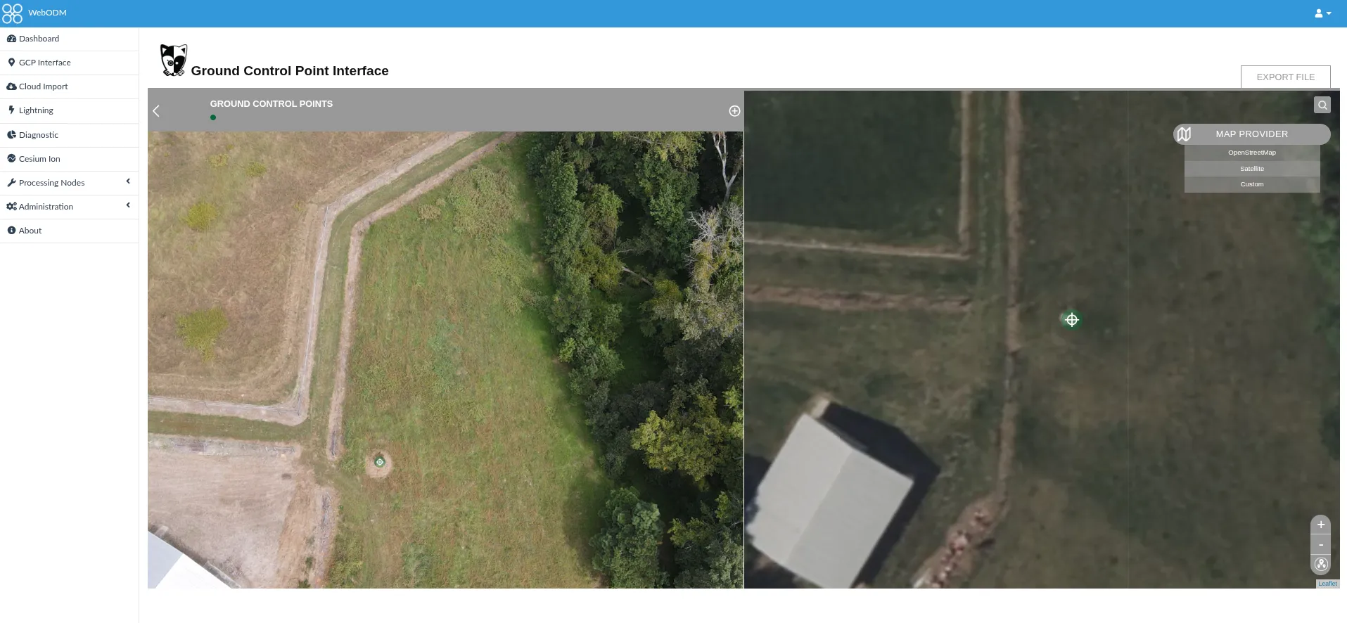
The WebODM documentation recommends at least 5 GCPs on 3 or more photos each. This data set has 3, the same as in Metashape, so expect a warning in the task log; processing still uses them. The resulting gcp_list.txt has one line per GCP per photo: coordinates, pixel position, file name, label.
Stage 2: Processing
Create the task
Click Select Images and GCP on your project and select the 78 photos plus geo.txt plus gcp_list.txt. WebODM recognizes the two text files by name.
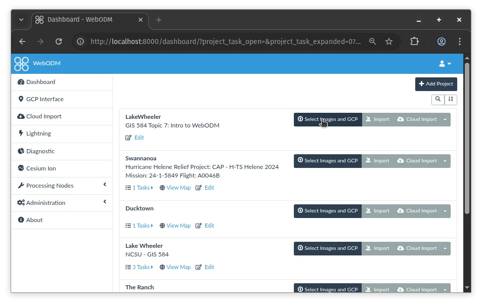
Give the task a name, keep the default processing node (node-odm-1), and choose the DSM+DTM preset. Click Edit to check the options:
dsm: true,dtm: truedem-resolutionandorthophoto-resolution: leave the defaults (5 cm/pixel; they are capped at the ground sampling distance)pc-quality: medium(the default), comparable to Metashape’s Medium point cloud- Leave resize images at the default
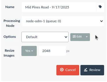
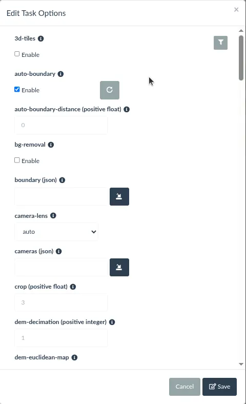
Click Review, check the summary, then Start Processing. Note the start time.
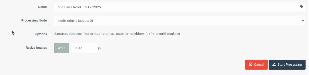
Processing takes from twenty minutes to a few hours depending on your hardware and, with Docker, on how much CPU and memory Docker Desktop is allowed to use (Settings, Resources).
Monitor
The task shows its progress and console output on the dashboard. When it finishes, the task card lists the number of reconstructed points, the average GSD, the area, and the processing time.
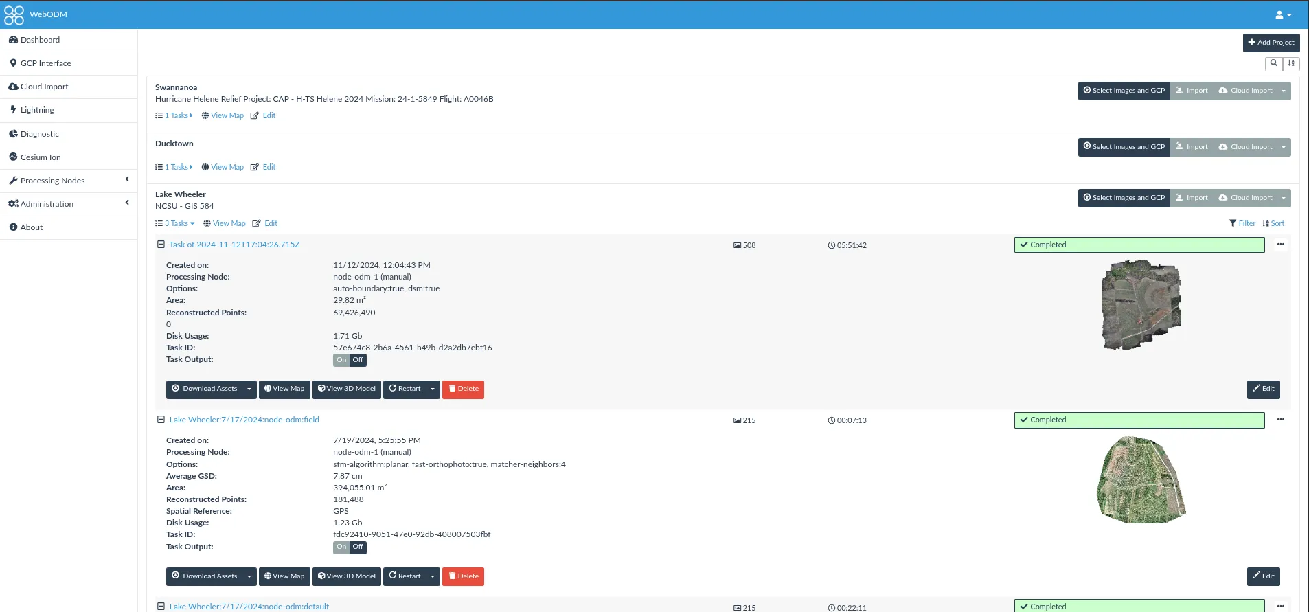
If a task fails or you change an option, Restart lets you resume from a later pipeline stage instead of starting over.
Stage 3: Results and export
View
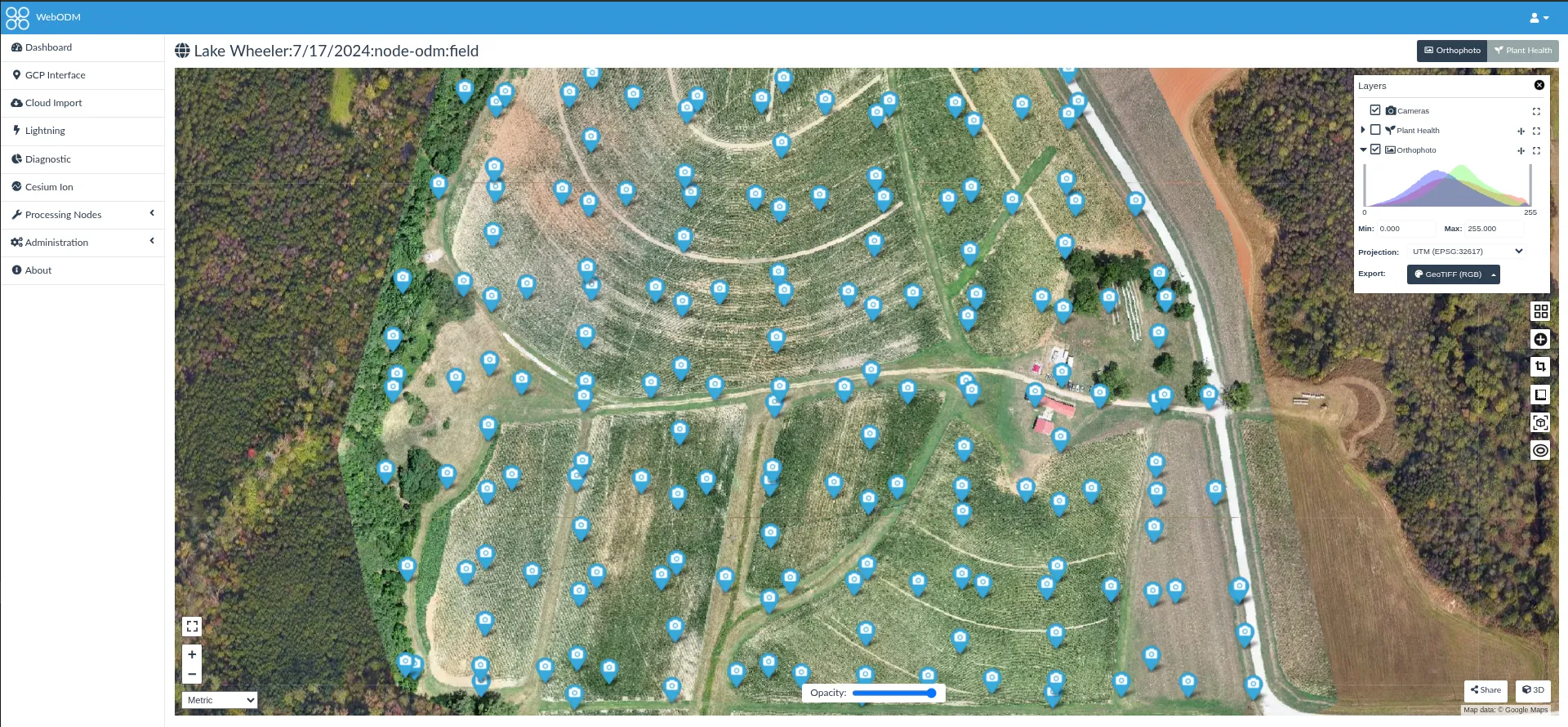
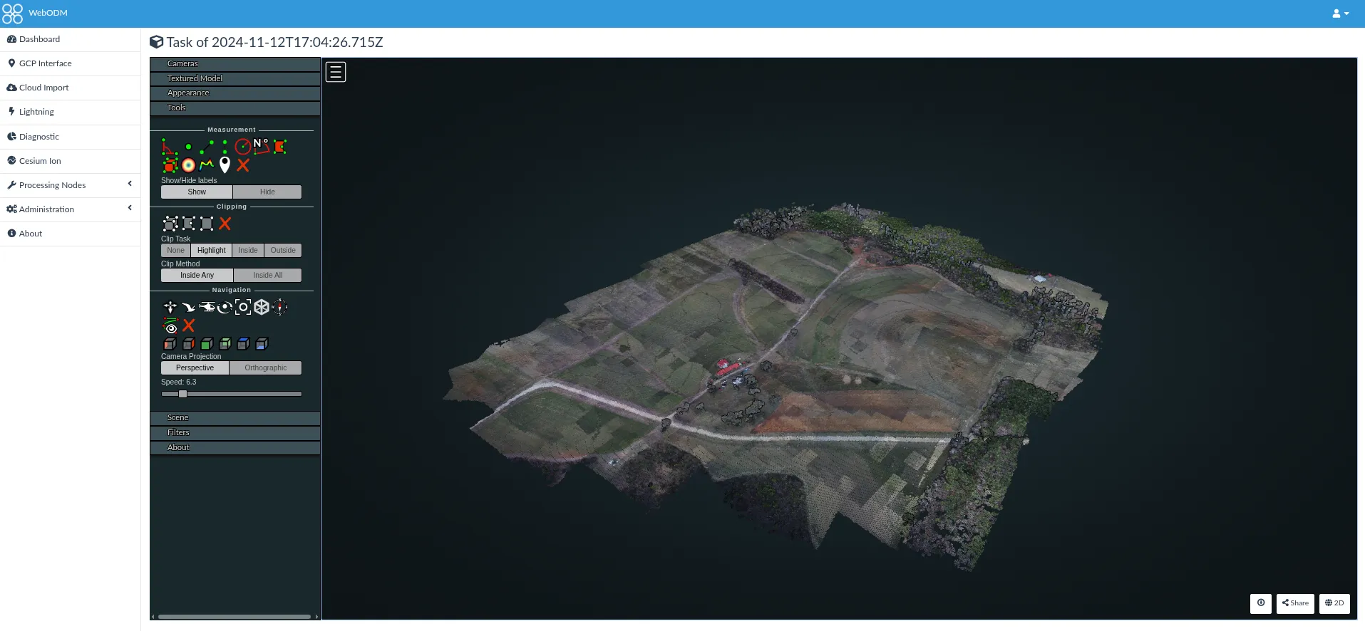
View Map opens the orthomosaic with the DSM and DTM as switchable layers and a measurement tool; View 3D Model opens the point cloud and textured model.
Download
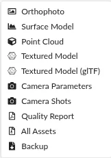
Download Assets offers each product separately or everything as one zip:
- Orthophoto (GeoTIFF)
- Surface model (DSM) and terrain model (DTM), GeoTIFF
- Point cloud (LAZ)
- Textured model
- Quality report (PDF): the WebODM equivalent of the Metashape processing report, with GSD, overlap, camera calibration, and the GCP errors
- Backup: the whole task, to reload into another WebODM instance
Stage 4: Compare with Metashape
Then look at:
- Orthomosaics side by side at building edges, tree crowns, the road, and the field boundary: sharpness, seams, doubled or smeared features, extent.
- Quality report versus processing report: GSD, number of reconstructed points, GCP errors, and processing time.
Report
Prepare a report (3 to 5 pages including figures):
- Setup: your machine and installation route, the task options, and the processing time; the photos on which you marked each GCP.
- Products: figures of the WebODM orthomosaic and DSM with their coordinate system and cell size.
- Comparison: the side-by-side figures, the DSM difference statistics and map, and the report figures from both tools (GSD, point count, GCP errors).
- Discussion: which product you would trust more and why, and what each tool made easy or hard. Refer to the pipeline stages from Lecture 2B when explaining a difference.
Submission
Assignments 2B and 2C are submitted together as one combined report, due on the same date. Upload to Moodle, Assignment 2C:
- Your report as a PDF, with the WebODM quality report attached or included as an appendix.
Grading
- Products: orthomosaic and DSM shown, georeferenced, and described.
- Comparison: the two tools are compared with figures and numbers.
- Discussion: differences are explained with the processing concepts from the lectures.
- On-time submission.